


Chapter 2 Gravity and Dark Matter
2.1 The Two Body Problem
Kepler stated three laws of planetary motion:
-
planets move on ellipses with the Sun at one of the foci
- the area swept out in a unit amount of time by the line joining the Sun to the planet is constant
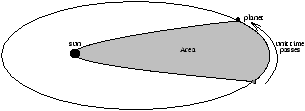
Figure 2.1 - Kepler's Second Law
- T2=ka3 where T is the orbital period, a is the average distance from the Sun and k is some constant
The general two body problem solves for the motion of two masses under their mutual gravitational interaction for arbitrary values for m1 , m2 , r1(0) , r1(0) , r1(2) and r2(0) .
2.1.1 General Coordinate Consideration
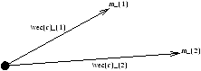
Figure 2.2 - Gravitational Force Between Two Bodies
there is no net force as
F=F12+F21=0=m1r1+m2r2
which we integrate to form
m1r1+r2=c
and again
m1r1+m2r2=Ct+D=(m1+m2)rC
therefore the centre of mass defines an inertial frame which refers the centre of mass frame which sets
C=D=0
Þ m1r1+m2r2=0
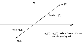
Figure 2.3 - The Centre of Mass Frame
In addition the motion is confined to a plane which is defined by r1(0) and r1(0) .
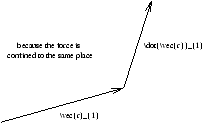
Figure 2.4 - Motion Confined to a Plane
we now consider that the motion of m2 is
we know that
and so we can rewrite our previous equation as
so we can say that
and we find the acceleration is
similarly this can be found for m1
where
2.1.2 General Solution for Circular Orbits
| a=r1+r2=r2 |
æ
ç
ç
è |
|
+1 |
ö
÷
÷
ø |
=r2 |
|
2.1.3 Applications of Circular Orbits and Solutions
Visual Binaries
The ideal case for a Visual Binary Orbit is in the plane of the sky
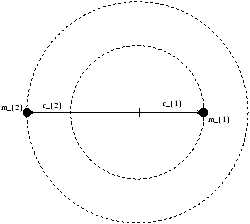
Figure 2.5 - A Visual Binary Orbit System
we measure r1 , r2 and T so that we can work out
and also that
which provides us with two simulateous equations which permits us to calculate m1 and m2 .
2.1.4 Spectroscopic Binaries
Spectra of Both Stars Measureable
Initially we will be assuming that the plane of orbit is edge on so we observe the full componment of radial motion. This is where the inclination is 90°
m1r1+m2r2=0
m1r1+m2r2=0
m1v1=m2v2
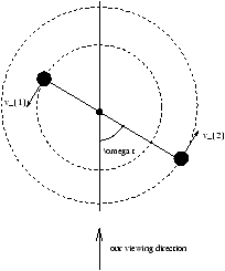
Figure 2.6 - Our View of the Remote System
we measure the radial velocities
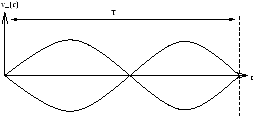
Figure 2.7 - The Radial Motion of the System
now
now using Kepler's Third Law
now by combining our results of the above and m1v1=m2v2 we obtain an equation that allows us to obtain the mass of the stars
However if the plane of orbit is inclined at an angle i then we only measure
v1sini=v1'
v2sini=v2'
where we only can measure v1' and v2' . Therefore we get
but if i is unmeasureable there is an uncertainity of sin3i in the measurement of the masses.
In eclipsing binaries we know that sini~ 1 .
Only One Spectrum is Visible - Planet Finding
The first planet discovered was by Mayor and Queloz (1995 - Nature 378,355). From the previous subsection
m1v1=m2v2
m1v1'=m2v2'
and rearranging this gives
The Right Hand Side of the above equation is the observarable part of the mass function. This is currently the best method for detecting planets. From spectroscopy we can determine the type of star and hence its mass ( m1 ). For planets m2<<m1 so
The Left Hand Side is what that can be determined.
Considering the detectability
If we take Jupiter as an example
T=11.9 years
m2=1.90× 1027kg
v1'=12ms-1
Jupiter is just detectable as the current limit is about 10ms-1 for v1' .
Solution of the General Two Body Problem
Acceleration in Plane Polar Coordinates
Motion is confined to a plane so it is sensible to use the plane polar coordinate system.
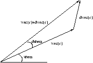
Figure 2.8 - Acceleration in Plane Polar Coordinates
we now use the unit vectors lr and lq as the unit vectors in the radial and tangential directions.
r=rlr
Þ r=rlr+rlr
we now look at the change in the unit vector
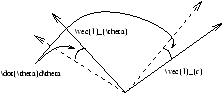
Figure 2.9 - Considering the Change of The Unit Vectors
differentiating again
where (r-rq2)lr is the radial acceleration and (2rq+rq)lq is the tangential acceleration.
By applying this we can get the equations we need to solve for our two body problems
By using Kepler's Second Law we start off with
rq+2rq=0
and we integrate
r2q=constant=h
however
r2q=2× (rate of sweeping)
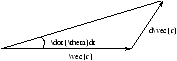
Figure 2.10 - ???
this is a result of the central force, which leads to the result of Kepler's Second Law.
Another view would be to introduce h
h=r×r
differentiating this gives us
mh=0
mh=constant=mr×r=L=angular momentum
or this can be interpreted that Kepler's Second Law just states that angular momentum is conserved.
Ellipse in Plane Polar Coordinates
in cartesian coordinates an ellipse is
an ellipse is a locus of points such that the sum of the distance to the two foci is fixed. An ellipse can be fully specified by two numbers.
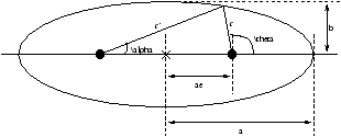
Figure 2.11 - An Ellipse
where a is length of the semi-major axis ( b is the semi-minor axis) and e is the eccentricity.
r+r'=2a
r+r'=a-ae+a+ae
rcosq+2ae=r'cosa
rsinq=r'sina
r2cos2q+4a2e2+4aercosq+r2sin2q=r'2
r'=2a-r
r'2=4a2-4ar+r2
r2cos2q+4a2e2+4aercosq+r2sin2q=4a2-4ar+r2
however r2=r2sin2q+r2cos2q so
4a2e2+4aercosq=4a2-4ar+r2
recosq+r=a(1-e2)
in general e can be greater than one which makes the ellipse equation form a conic section.
Figure 2.12 - Conic Sections
The closest approach where q =0 then r=a(1-e) which is known as the perigee. The furthest approach where q =p is where r=a(1+e) is known as a apogee. This leads to b=a(1-e2)1/2 .
The General Solution and Kepler's Third Law
| |
é
ê
ê
ë |
eg. for r2, M'= |
|
ù
ú
ú
û |
r2q=h
we write this as
we use the substitution u=1/r and also conservation of angular momentum dq/dt=h/r2=hu2
we differentiate once
and then differentiate again
| |
|
æ
ç
ç
è |
|
ö
÷
÷
ø |
= |
|
=-h |
|
æ
ç
ç
è |
|
ö
÷
÷
ø |
=-h |
|
|
æ
ç
ç
è |
|
ö
÷
÷
ø |
We need two equations
-
at=-GM1M2/2E (Problem Sheet 1, Question 6)
where at=a1+a2
- GM'/h2=1/a(1-e2)
now the total angular momentum is
L=m1h1+m2h2=m1r12q+m2r22q
by using m1r1=m2r2 the second equation can be tidied up after lots of crunching to obtain
now by using the first equation we get
for a given L and E we can compute at and e , for example
and the orbit is
We notice that when E=0 that at=¥ and e=1 so when E<0 then e<1 occurs and we get a bound orbit (ellipse/parabola). However when E>0 then e>1 and so we have a unbound orbit which is a hyperbola.
General Form of Kepler's Third Law
The area of an ellipse is
the rate of sweeping is
by squaring the rate of sweeping we get
for example for r2
this can be manipulated to obtain
This is Kepler's Third Law in its general form.
2.2 Galaxy Rotation Curves
The sun rotates around the centre of our galaxy, the Milky Way, at about r=8.5 kpc and speed vc=220kms-1 (which is the circular speed). In the Milky Way the circular speed is approximately constant with radius. In other large spiral galaxies the rotation curve is approximately flat and can be measured well beyond the extent of the optical light ( ~ 10kpc ) with radio measurements ( ~ 40kpc ).
In we consider that the galaxies act like point masses we get
however a measurement of the mass gives figure 2.13
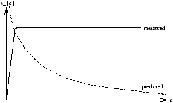
Figure 2.13 - Measured/Predicted Mass Distribution of a Galaxy
Figure 2.13 shows us that most of the mass cannot be concentrated neat the galaxy centre even though most of the light is within 10kpc . A more sophisticated model is the stella light method
a typical rs is 3kpc . Computing vc for this mass distribution it peaks at 2.2rs , beyond 3rs the point mass model is good enough.
Another technique to measure the mass of points on a galaxy is to look at the oscillating acceleration of the stars, their vertical motion, as in figure 2.14
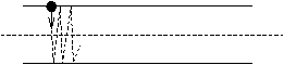
Figure 2.14 - Vertical Oscillating Acceleration
If there is more mass in the section of the disk then the acceleration of the stars on the top/bottom of the galaxy is much greater. This is the basis of calculating the mass at certain points through the galaxy. If this is done then we it tells us that what we see makes up the galaxy is what is there.
So we postulate a dominant spherical distribution of dark matter (of unknown form) to explain the rotation curve. What is r (r) for the galaxy? For a spherical distribution only M(<r) has gravitational effect and so acts as if at r=0 .
| M(<r)= |
ó
õ |
|
r (r')rp r'2dr' |
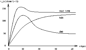
Figure 2.15 - NGC3198
The disk mass, computed from the light, is about 3.4× 10¹⁰M . Because for the halo
therefore the total mass inside r<30kpc is
| M(<30kpc)=Mdisk× |
|
=1.6× 10¹¹M |
|
we recall for ??MW?? that Mstar~ 1× 10¹¹M
within 100kpc we find that
so we can conclude that in spiral galaxies that most of the mass is in the form of dark matter. This matter is distributed with the density of
which out to the limits of measurement show that
since Mµ r we don't really know the masses or what their sizes are.
2.3 The Virial Theorem
For a planet in a circular orbit around a star
2T=-U
where T is the kinetic energy and U is the potential energy. More generally for a binary star
<2T>=-<U> (where <x> is average of x)
This is covered in Problem Sheet One, Question 7.
The Virial Theorem states for any gravitationally bound system in a steady state equilibrium then, then the time averaged kinetic energy is equal to minus the time averaged potential energy.
Þ <T>=-<U>
An alternative formalation of this is
E=T+U
so the total energy is half the potential energy.
The Virial Theorem is a powerful tool for measuring masses on different scales, from star clusters to galaxy clusters.
Consider a bound collection of masses, in an inertial frame where the centre of mass is stationary.
now
| 2T= |
|
mir |
i= |
|
|
(ri.mir |
i)- |
|
ri.miri |
To prove this we will consider three points
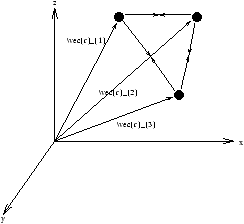
Figure 2.16 - The Appication of the Virial Theorem on Three Points
| |
|
ri.Fi=r1(F12+F13)+r2(F21+F23)+r3(F31+F32) |
~iri.Fi=r1(F12+F13)+r2(-F21+F23)+r3(-F31+-F32)
~iri.Fi=(r1-r2).F12+(r1-r3).F13+(r2-r3).F23
| ~iri.Fi=-r12. |
|
r12-r13. |
|
r13-r23. |
|
r23 |
~iri.Fi=U
but steady state implies that
å Ai(t)~å Ai(0)
so that for a large enough t then
2<T>=-<U>
For a relaxed body with a large number of component stars/galaxies, T and U are constant so we don't need to do any time averaging. This permits us to simply write
2T=-U
This is the most useful form of the equation as no time averaging is involved.
2.3.1 The Application and Assumptions of the Virial Theorem
Kinetic Energy
We will assess this in three stages
-
consider a cluster of N visible stars of equal mass M
now in a similar technique to that which is used in Thermodynamics
<v2>=<vx2+vy2+vz2>
<v2>=<vx2>+<vy2>+<vz2>
Þ <v2>=3<vx2>
this is true for a spherical symmetric system
where s is known as the one dimensional velocity dispersion which is the root mean square of vx which also is the standard deviation of the radial velocity relative to the mean.
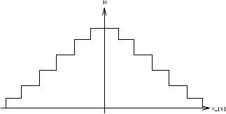
Figure 2.17 - Distribution of the Velocity
- the cluster contains stars with a range of different masses ( m1, m2, ... ), these contribute
| T=T1+T2+... = |
|
s12+ |
|
22+... |
- some of the stars are invisible, however this doesn't change the equation and so it is still
this is because the visible and dark matter mass have the same distributions (an assumption)
Potential Energy
-
Example One:
- a sphere of uniform density r , radius R so that the mass is
to compute the potential energy ( U ) we consider assembling in shells where we add shell by shell of thickness dr
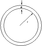
Figure 2.18 - Shell Adding to Calculate Potential Energy
however M(<r)=4/3p r3r so
but M2=16p2/9R6r2
if we now apply the Virial Theorem
2T=-U
so all we need to do is observe what s and R is to be able to obtain the mass M
- Example Two:
- via the observations of galaxy clusters (Carlberg et al 1996, Astrophysics Journal 462, 32), in this example we will be looking at galaxy cluster A2390 which has:
s =1093 kms-1
r=4.5Mpc
from the observations of the light profile we can derive the virial mass
the mass in the stars is
a typical value for a galaxy cluster is 60. The scale of this is some large that this is believed to reflect the Universal Value.
Wm=0.3
2.4 Gravitational Lensing
There is really only one equation in this aspect of physics (for the weak gravitational limit, ie. not near a black hole), a photon with an impact parameter of R is deflected through an angle a
this is what Einstein postulated in 1915, it was double the size of the classical value. The weak field is when R>>RS where RS is the Schwarzchild radius which is
for the Sun RS=3000m and at the Sun's limit a=1.75'' . For all astrophysical objects except a black hole RS<<R
Þ a~ 1''
we can therefore use small angle approximation
sinq=tanq=q
we can treat light as travelling in straight lines which have been bent as it passes an object
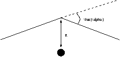
Figure 2.19 - The Basics of Gravitational Lensing
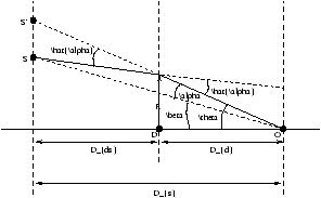
Figure 2.20 - Gravitational Lensing
2.4.1 The Lens Equation
We consider the plane defined by the source S, the deflector D (star/galaxy) and the observer O. The line OS defines the optic axis, the ray from S and going towards O is in the plane SDO. The lens equation is a statement of the geometry
AS=AS'-S'S
Dsb =Dsq -aDds'
We note that normally Ds=Dds+Dd however this is not true at cosmological distances
and these cosmological angular diameter distances relate the transverse distances to their angles.
The lens equation simply says
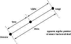
Figure 2.21 - The Lens Law, Viewing End On (View on the Sky)
the problem is to solve for q (the image position), given b (the source position).
2.4.2 Solution for the Point Mass
we know that
and so we rewrite the lens equation as
however Dds/DdDs=qE2 so
q2-bq -qE2=0
so there are two solutions and two images, this corresponds to one above the optic axis and also there is one below it.
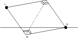
Figure 2.22 - Solutions for the Point Mass
when b =0 then q =±qE and this is for the perfect alignment case which forms a ring image of angular radius qE . This is known as an Einstein Ring.
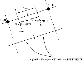
Figure 2.23 - The Two Solutions as Seen on the Sky
2.4.3 Images and Parity for a Point Mass
If we consider a source (eg. a galaxy) which has a finite angular size and shape
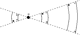
Figure 2.24 - Images and Parity for a Point Mass as Seen on the Sky
Figure 2.24 shows a series of dots ( · ), empty circles ( ° ) and crosses ( × ), these represent what unique parts of the image form where. This is in accordance with the lens equation.
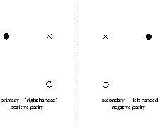
Figure 2.25 - Primary and Secondary Imaging (Parity)
2.4.4 Magnification
We define the solid angle (the steradian) as:
-
steradian:
- is the angular area l extended
the units of the are (radians)2 (or called steradians)
for example the solid angle of the whole sky is
or another example is a square galaxy with dimensions (ra )× (rb ) then
W =ab
Back to magnification, in lensing the surface brightness is preserved, so lensing magnifies objects (increases their solid angle) so that
(magnification) = (flux amplication)
by using figure 2.25 (redrawn with relevent information as figure 2.27) we can work out the magnification
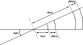
Figure 2.26 - Calculation of the Magnification
the area of the source is rb df db (here r=DS ) and so the solid angle of the source is b db df . The area of the image is rq df rdq (here r=Dd ) and so the solid angle is q df dq . The magnification is
| M (magnification)= |
|
= |
½
½
½
½ |
|
|
½
½
½
½ |
u=1 Þ M=1.34
u=0 Þ M=¥
[u=0.8266 Þ M=1.5]
2.4.5 Solution for Extended, Circular Symmetric Masses and Young Diagrams
For a galaxy we can use the thin lens approximation, this is because Ds (etc)>>rgalaxy .
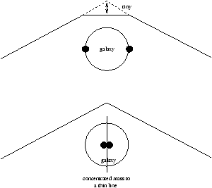
Figure 2.27 - The
Thin Lens Approximation for a Galaxy
We now need to calculate a(q ) due to the projected mass distribution. If the projected mass distribution is circularly symmetric then we only need to consider M(<R) to be concentrated to a point ( R=0 ) and then ignore M(>R) . Therefore
then we apply the lens equation
however this is a non-linear equation. So to solve this we use a graphical technique by writing that there are two relations between a and q
-
a =q -b
- a =4GM(<q )Dds/c2DdDsq=f(q )
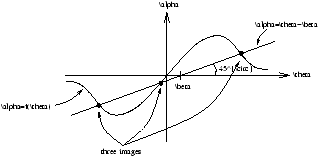
Figure 2.28 - The Young Diagram - The Graphical Solution