

Chapter 1 Contents of the Universe
1.1 Coordinate System
We need two planes that define the two dimensional coordinate systemso a recording of locations can be made onto the celestrial sphere. The plane of the Earth's equator which is the orbit about the Sun and is know as the ecliptic.
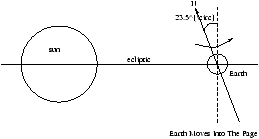
Figure 1.1 - The Plane of the Ecliptic
If we projected lines of latitude this is known as Declination, projecting lines of longitude is known as Right Ascension.
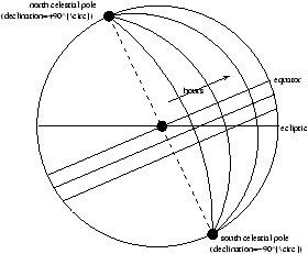
Figure 1.2 - Our Coordinate System
Zero Hour is where the ecliptic intersects the equator. The Right Assension is measured in hours, minutes, seconds (where 24 hoursº 360° ). Declination is measured in degrees, arc-minutes ( (1/60)° ) and arc-seconds ( (1/3600)° ).
The changing apperance of the night sky, and the seasons, are explained by this picture. The Siderial day is shorter than the Solar day by about four minutes.
The Earth's axis precesses with a period of 26000 years so the coordinate syste, has to be recalibrated as it is constantly changing.
1.2 Solar System
Some basic numbers
| Planet (Jehovian) |
d (AU) |
e |
M ( MJ ) |
T (years) |
Year Discovered |
Discovered By |
| Mecury |
0.39 |
0.21 |
1.7× 10⁻⁴ |
0.24 |
|
|
| Venus |
0.72 |
0.01 |
2.6× 10⁻³ |
0.62 |
|
|
| Earth |
1 |
0.02 |
3.1× 10⁻³ |
1 |
|
|
| Mars |
1.52 |
0.09 |
3.4× 10⁻⁴ |
1.88 |
|
|
| Jupiter |
5.2 |
0.05 |
1 |
11.9 |
|
|
| Saturn |
9.54 |
0.06 |
0.3 |
29.5 |
|
|
| Uranus |
19.18 |
0.05 |
4.6× 10⁻² |
84 |
1781 |
Herschel |
| Neptune |
30.06 |
0.01 |
5.4× 10⁻² |
16.5 |
1846 |
Adams, Levemer, Salle |
| Pluto |
39.44 |
0.25 |
6× 10⁻⁶ |
249 |
1930 |
Tombaugh |
| |
Arstarchus in 280BC was able to measure the distance to the Sun, he knew that the Sun was much further away than the Moon. He also devised a heliocentric solar system model (everything revolves around the Sun), not as a solid theory but as a way of looking at our solar system.
Eratoshenes who lived between 276-195BC found the radius of the Earth (not everyone believed the Earth was flat) and in AD140 Claudius-Itolemy put forward a geocentric model where everything revolved around the Earth. It wasn't until 1473-1543 where Copernicus devised a heliocentric model. Although Copernicus was correct he assumed that the planets moved in circular orbit (not eliptic as they do) so he still had to resort to epicycled orbits. When he put forward his model the Church at the time had adopted the geocentric model so that when he published his model there was a lot of heavy opposition, it didn't help that his model needed the epicycles.
Between 1546-1630 a Danish Observer called Tycho Brahe whose measurements were highly accurate so when he published them, Kepler (1571-1630) could devise his three laws, however they were derived completly by emperical methods. After Kepler formed his three laws, Newton (1642-1727) was able to provide an explanation of Kepler's laws by his law of gravity which relies on the inverse square law for the magnitude of the force ( 1/r2 ).
1.3 The Milky Way
Distances are generally measured in Parsecs (pc) (this will be covered in chapter 3). A Parsec is about 3.086× 10¹⁶ m=3.26 lyr . The typical distance between stars is generally one parsec (our nearest star is Proxim Centauri which lies about 1.31 parsecs away). Stars can have temperatures in the range 2000<T<100000K and their mass can range over 0.08M<M<100M .
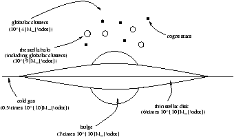
Figure 1.3 - An Overview of a Galaxy
The circular velocity of the galaxy is about 220 kms-1 and the age of the oldest star is 12× 109 years (we are quite a young solar system when compared on the great scale). The mass of a volume of radius 50 kpc is about 5× 10¹¹ .
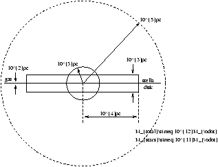
Figure 1.4 - An Cartoon Spiral Galaxy
1.3.1 History of The Discovery of the Milky Way
-
1610:
- Galileo resolves the Milky Way into stars
- 1785:
- Herschel'l makes his star map
- 1923:
- Hubble measures the distance to the Andromeda galaxy
- 1930:
- Trumpler makes an anaylsis of the absorption of light by dust
1.4 Galaxies and Clusters of Galaxies
The nearest galaxy that is large is called Andromeda (M31) and it lies about 700 kpc away. The typical spacing of galaxies is about 1 Mpc and the normal range of the mass of a galaxy is 107M<M<1012M . Basic types of galaxy exist, spirals (disk) and ellipticals (smooth). Blue stars are stars forming and the red ones are inactive stars.
Galaxies are not distributed randomly throughout the universe but instead show a hierachy of clustering. The nearest galaxy cluster is Virgo and its distance is about 17Mpc . Galaxy clusters can contain anything in the range of fifty to thousands of galaxies with mass in the region 1015 M . The scale of these cluster's is typically about 5 Mpc .
1.5 Cosmology
Cosmology is the science of the Universe. If began in 1915 when Einstein completed his theory on General Relativity. In 1929 Hubble discovered that the Universe is expanding and in 1965 Cosmic microwave background radiation was discovered. Finally in 1998 it was found that there was a Cosmolgical constant, it has been measured however there is some uncertainity about its meaning.
We define the redshift as
This can be interpreted a Doppler Shift which is described by the equation
Hubble's Law is that the velocity is proportional to distance
Þ cz=H0d=v
where v is the velocity of recession and H0 is Hubble's Constant which is about 70± 10 kms-1Mpc-1 . Sometimes it value is given in different units.
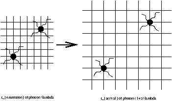
Figure 1.5 - The Red Shift in Action
(1+Z) is the factor by which the Universe has expanded between the time of emission temission and tarrivial .
1.5.1 A Mathematical Description
The mathematical description of the Universe combines Einstein's General Relativity theory with the Copernican principle. The Universe on a large scale is isotropic (the same in all directions). If we do not inhabit a special place (as stated in the Copernican principle) it must be homogeneous (the same everywhere). This results in all observers see the same in the big picture. The behaviour is governed by two parameters, H0 (the Hubble Constant) and W0 (the density parameter).
The density parameter ( W0 ) is equal to
where r0 is the current density and is about 1.88× 10⁻²⁶ h2 kgm-3 .
W0=1 is the boundary between the cases where the Universe will eventually recollapse or expand forever.
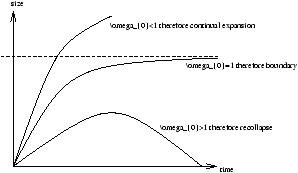
Figure 1.6 - The Outcomes of
W0
As we look out further we look back at shells of successively older times. At small distances
however at large distances (large redshifts)
By looking back to where z=1000 we look back to the early times of the Universe, when it existed in a plasma state (when the Universe was opaque). It is this level of redshift that makes up the cosmic microwave background radiation (CMB). The distance to the shell that makes up this level of background radiation is
The observable universe contains around 1012 galaxies, the attempt to try and see more is impossible as this CMB barrier is opaque. By measurement the density in this CMB we can see what the structure of the universe was like at a young age.
Recent observations (1998) of supernovae provide rather compelling evidence for a third cosmological parameter L0 and is known as the Cosmological Constant. This constant provides a force of repulsion, it comes as a consequence of the energy density of a vacuum and is the constant of integration in Einstein's Field Equations.
1.5.2 Summary of Current Estimates
Summarising the current estimates of the contents of the universe
Wvisible=0.01 visible matter
Wb=0.03 baryonic (normal) matter
Wm~ 0.3± 0.1 exotic matter
1.6 Observing the Universe
The principle windows for ground based astronomy are:
-
optical and near infrared
320nm® 2300nm
- radio
10-2m® 10m
other regions are either grotty or impossible to observe from the ground and so need to be observed from outside the Earth's atmosphere.
Astronomers divide up the electromagnetic spectrum as follows
l
| g -rays |
<0.1nm |
high energy processes (eg. black holes) |
| X-rays |
0.1nm® 10nm |
high energy processes (eg. black holes) |
| ultraviolet (UV) |
10nm® 300nm |
|
| optical |
300nm® 1000nm |
stars |
| infra-red |
10-6m® 10-4m |
molecular dust |
| microwave |
10-4m® 10-3m |
molecular dust |
| radio |
10-2m® 10m |
charged particles in magnetic fields |
| |
we will mostly be studying the optical part of the electromagnetic spectrum. Stars have spectra that can be approximated to a black body and they generally peak in the optical to the near infra-red.
Wien's Law states that
for example the hottest star which has a temperature af about 100,000K peaks at around 29nm , a typical star ( 5000K ) at around 580nm and the coolest star ( 2000K ) is around 1450nm .
Luminosity is defined as
Lº power Js-1
and for a black body its
L=s AT4
Consider the the problem of planet detection by reflected or re-radiated light, all the stars even the nearest are unresolved (eg. a sun at 5pc )
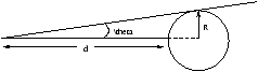
Figure 1.7 - Resolving Star
| q =4.5× 10⁻⁹× |
|
× 3600=10-3 '' |
The brightness of a planet is defined by the flux it emits, this is measured in energy per sec incident on per unit area. So that at a distance d
the energy intercepted by a planet per sec
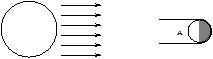
Figure 1.8 - Brightness of a Planet
the reflected luminosity is
where a is the albedo for the earth ( a=0.35 ).
for example an Earth like planet which is 1AU from the star
Needless to say not very bright!
The lumionity absorbed and re-radiated is
| Lp'=s 4p rp2Tp4= |
|
= |
|
s 4p rS2TS4 |
Using Wien's Law
which lies in the mid infra-red.
we can show that the signal to noise ratio is
so we need a long time ( t ), large area ( A ), small distance ( d ) and high resolution to observe a planet.
For a solution that is more plausible we need the NASA Terrestrial Planet Finder which has a baseline of 1000m (http://tpt.jpl.nasa.gov/)
1.7 Magnitude of Brightness
Hipparchus in 140BC gauged the brightness of stars by eye on an apparent scale ( m ). This scale has a range of one to six, where one is the brightest star and six is one that is just visible by the naked eye.
same difference in mº same flux ratio
for example
we find that the difference between brightness magnitude one and six is of the order of about 100 so
1-6=-klog100
Þ k=2.5
k is known as Pogson's definition, so in general we can write
m=C-2.5logf
1.7.1 The AB Magnitude System
Measuring the brightness with the previous equation is fine until we wish to measure brightness at different wavelengths.
where fn is the flux per unit frequency and so measured in Wm-2Hz-1 . For example a hypothetical star of apparent magnitude zero
In practice we integrate over a filter
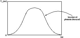
Figure 1.9 - Brightness Through a Filter
The detected flux is
the magnitude therefore is
we write down the standard band passes in the optical window in the following mannor
-
U is Ultra Violet
- B is Blue
- V is Green
- R is Red
for example
mB=B=CB-2.5logfB
mV=V=VV-2.5logfV
However our eye is not the best device for detecting faint stars. The Hubble Space Telescope can measure is V~ 29 therefore
| 23=-25log |
æ
ç
ç
è |
| f(Hubble Space Telescope) |
|
| f(eye) |
|
ö
÷
÷
ø |
|
| Þ |
| f(Hubble Space Telescope) |
|
| f(eye) |
|
=10 |
|
=6.3× 10⁻¹⁰ |
1.7.2 Absolute Magnitude
The Absolute Magnitude ( M or MB )is the apparent magnitude that would be measured for a star at ten parsec's.
| Þ m-M=-5log |
|
(for when d is in parsecs) |
1.7.3 Colour
Colour is the measure of the difference of the brightness magnitude at different wavelengths. For example
this provides us with a logarithmic measurement of the flux ratio.
1.8 Distances In The Universe
1.8.1 Trigonometric Parallax
Due to the Earth's orbit about the Sun a nearby star appears to wobble relative to a very distant background star.
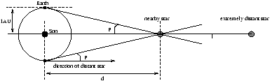
Figure 1.10 - Parallax Distance Measurement
so the angular shift is ± p=1 AU/d therefore
when p is one arcsecond ( p/180× 3600 rad ) then d is one parsec
therefore we can simply state that
the first parallax measured was by Bessel in 1834 and it was of the star 61 Cygni which he measured p=0.29'' which translates to a distance of about d=3.4 parsecs . Today we have measured parallax's for 120,000 stars in a range of about 200 parsec's with the satelite Hipparcos.
1.8.2 Cepheid Variable Stars
Leavitt in 1912 discovered that the period of a star is related to its absolute magnitude.
so to obtain the distance we measure the period to obtain the absolute magnitude and then use
so a quick calculation shows that for M=-4 and m=28 gives a distance of about 20 Mpc with an error of about 10% (with the Hubble Space Telescope).
1.8.3 Type la Supernovae
White dwarfs accreting from a companion explode when they reach the Chandrasekhar limit, this limit lies at about when the white dwarf has a mass of about 1.4 times more than our Sun . As this is a physical critical limit all white dwarfs explode and emit light in the same way and quantity. This provides us with something to calibrate our measurements against. The peak brightness of the explosion is related to the shape of the light curve so there is a relationship between absolute magnitude and the tdecay . As we can measure the apparent magnitude and we can calculate the absolute magnitude from the rate of decay in the light curve we can measure distances up to about 5× 10⁹ pc with an accuracy of about 10% (due to measuring the apparent magnitude to an accuracy of about 0.2). This distance is approachingthe size of the observable universe.
1.8.4 Summarise
| Method |
Distance |
| Parallax |
d=200pc=2× 10² |
| Cepheid |
d=20Mpc=2× 10⁷ |
| Supernovae |
d=5Gpc=5× 10⁹ |
| |