


Chapter 6 Boltzmann's Entropy
what is the microscopic origin of S ? The properties of S are
-
Second Law gives us that D S³ 0
- S is a maximum at equilibrium
- SAB=SA+SB
- Third Law says that S=0 when T=0
S=S(U,V,N)
Boltzmann's proposal was that S=klnW where W was the number of microstates required to build a macroscopc state with a given U , V and N
- WAB=WA× WB
Þ SAB=SA+SB
- at T=0 , all systems go to the general state so typically this is W=1 which implies S=0
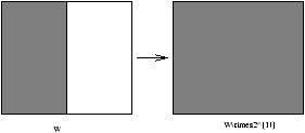
Figure 6.1 - States Avalibility
6.1 Two Level Systems
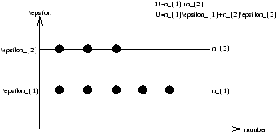
Figure 6.2 - A Two Level System
A macrostate is specified by n1n2 . What are the values of n1 and n2 at equilibrium
S=klnN
W is the number of different ways of arranging N particles, in level one and n2 in level two, so that N=n1+n2
|
W= |
æ
ç
ç
è |
|
ö
÷
÷
ø |
=NC |
|
= |
|
= |
|
(6.1) |
W=N(N-1)(N-2)
For large N and n1
lnN!~ NlnN-N (6.2)
S=k[lnN!-lnn1!-ln[(N-n1)!]]!
S~ k[NlnN-N-n1lnn1+n1-(N-n1)ln(N-n1)+N-n2]
S=k[NlnN-n1lnn1-(N-n1)ln(N-n2)
compare with dU=TdS-MdB
-
keep n1 and n2 fixed (so that dS=0 )
dU=n1de1+n2de2=(-n1+n2)µ dB=-MdB (as required)
- keep B fixed (so that e1 and e2 are fixed also)
dU=dn1e1+dn2e2=dn1(e1-e2) (N=n1+n2Þ dn1=-dn2)
compare this to TdS
| dS=k[-1-lnn1+1+ln(N-n1)]dn1=kln |
|
dn1 |
6.1.1 Calculation
| S=kN |
æ
ç
ç
è |
lnN- |
|
lnn1- |
|
lnn2 |
ö
÷
÷
ø |
| S=-Nk |
æ
ç
ç
è |
|
-lnZ |
ö
÷
÷
ø |
= |
|
+NklnZ |
TS=U+NkTlnZ
Þ F=U-TS=-NkTlnZ
this is known as the bridge equation. We now recall that
dF=-SdT-MdB
Þ F=F(T,B)
| S=- |
æ
ç
ç
è |
|
ö
÷
÷
ø |
|
, M=- |
æ
ç
ç
è |
|
ö
÷
÷
ø |
|
F=-NkTlnZ
this is true for large T (as we saw in section 4.6)
6.2 Microcanonical Ensemble for Gases
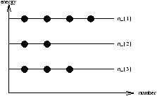
Figure 6.3 - ??
For fixed values of V and U=åSnSeS what are the values of nS at equilibrium? The energy levels for a box of gas molecules is
n=(nx,ny,nz), n2=nx2+ny2+nz2
where nx , ny and nz are discrete integer values ( 0 , 1 , 2 , 3 , etc).
Note that the energy levels are degenerate
-
many quantum states ( Y )
- have the same energy
for example n=(2,0,0) has the same n2 as n=(0,0,2) .
let gS be the degeneracy of levels (number of states with energy eS ). Also gS is the number of vectors n with fixed n2 .
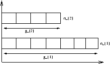
Figure 6.4 - ??
What is the equilibrium distribution of nS for fixed U , V and N ?
we use maximum entropy
S=klnW
where W is the number of ways of building a configuration with fixed nS . Maximise Entropy is subject to equations 6.5 and 6.6.
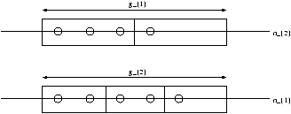
Figure 6.5 -
W For Two Levels
where g2n2 means that each particle g2 as so many ways of being in level two.
6.2.1 Computing W For Many Levels
where
where N=n1+n2+n3+...
Now we maximise entropy ( S=S(n1,n2,n3,... ) ) however n1 , n2 , n3 , ...are not independent.
so we need to solve
df+l df =0 (6.7)
| S=k[lnN! |
+ |
|
nSlngS |
- |
|
lnnS!] |
| S~ k[NlnN |
-N+ |
|
nSlngS |
- |
|
(nSlnnS-nS)] |
6.3 Equilibrium Values of **ns**
we maximise entropy
| f=lnW |
+a ( |
|
nS-N)-b ( |
|
nSeS-U) |
| d(lnW |
)= |
|
[lngSdnS-lnnSdnS] |
| df= |
|
(-lnnS+lngS+a -beS)dnS |
df=0ÞlnnS=lngS+a -beS
a and b are constants determined by
we now define the partition function as
Note that
6.4 Recovery of Thermodynamics
We derive dU=TdS-PdV
we recall that
this is because V=L3
this is if P=2/3U/V and only correct if U=3/2NkT .
The heat term, we recall
this is the condition for maximum entropy (and hence the equilibrium condition for nS ). We have solved
if T=1/b k ie. b =1/kT hence we get the funcdemental equilibrium of b
6.4.1 Computing S
S=klnW
| S~ k |
é
ê
ê
ë |
NlnN |
-N+ |
|
nSln |
|
+ |
|
nS |
ù
ú
ú
û |
| S=k |
é
ê
ê
ë |
NlnN |
+ |
|
nS |
æ
ç
ç
è |
-ln |
|
+beS |
ö
÷
÷
ø |
ù
ú
ú
û |
S=k[nlnN-NlnN+NlnZ+b U]
S=NklnZ+b kU
we recall that F=U-TS
U=NkTlnZ+U
Þ F=-NkTlnZ=-kTlnZN (6.12)
| F® P= |
æ
ç
ç
è |
|
ö
÷
÷
ø |
|
, S=- |
æ
ç
ç
è |
|
ö
÷
÷
ø |
|
6.5 Evaluation of Z
or we could write
where
so here degeneracy is automatically taken care of
| Z= |
æ
ç
ç
è |
|
C |
|
ö
÷
÷
ø |
æ
ç
ç
è |
|
C |
|
ö
÷
÷
ø |
æ
ç
ç
è |
|
C |
|
ö
÷
÷
ø |
F=-NkTlnZ
| F=-NkT |
æ
ç
ç
ç
ç
ç
ç
ç
ç
è |
lnV+ |
|
lnT+ln |
|
ö
÷
÷
÷
÷
÷
÷
÷
÷
ø |
|
S=NklnV+Nkln |
|
+ |
|
Nk+Nkln |
|
(6.14) |
| NklnV=Nkln |
|
+kNlnN-Nk+Nk=Nkln |
|
+Nk+klnN! |
lnN!~ NlnN-N
to make S extensive
S® S-klnN
since S=klnW we let W®W/N! [=WMB]
this is the corrected or maxwell-boltzmann counting for W . Dropping N! means permutations don't change physical state (see section 7 for an explanation). We note that this correction is not for localized particles (eg. paramagnetic systems).
With N! correction
|
S=Nkln |
|
+ |
|
NklnT+ |
|
Nk+ln |
|
(6.17) |
6.6 The Royal Route From Micro to Macro
Given a system where U , V and N is fixed
-
calculate the energy levels eS of each particle
- compute
- from free energy
F=-kTlnZN (localized)
-
| S=- |
æ
ç
ç
è |
|
ö
÷
÷
ø |
|
, P=- |
æ
ç
ç
è |
|
ö
÷
÷
ø |
|
-
U=F+TS
or
6.7 Localized Harmonic Oscillators
We have N simple harmonic oscillations in a heat bath of temperature T . This is a crude model of a solid. We apply the Royal Route
-
where s=0,1,2,... ,¥
-
where x=e-bw
-
F=-kTlnZN
since it is localized
-
-
| U=-N |
|
(lnZ)=-N |
|
æ
ç
ç
è |
- |
|
bw -ln |
|
ö
÷
÷
ø |
T® 0, b®¥ , second term® 0
T®¥ (kT>>kw ), b® 0 (6.20)
f=2 because there are two degrees of freedom
kinetic and potential energy gives one degree of freedom each, so the specific heat is
for one mole of substance
N=3NA
Þ c=3NAk=3R
this is known as the Dulong Petit Law
6.8 Diatomic Molecules
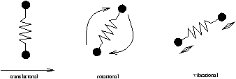
Figure 6.6 - Energy Stored in Diatomic Molecules
How do these three degrees of freedom combine?
e =et+er+ev
Þ Z=ZtZrZv (6.21)
F=Ft+Fr+Fv
therefore S , U and e all add for the translational, rotational and vibrational modes. eg
| cV=CVt+CVr+CVv= |
|
Nk+Nk+Nk= |
|
Nk (see Classwork 5) |