

Chapter 7 Quantum Statistical Mechanics
7.1 Validity of Classical Statistics
where
mkT~ (D p)2
where l is the themal de Broglie wavelength which is the uncertainity due to thermal and quantum effects.
|
e |
|
~ |
| quantum volume |
|
| volume per particle |
|
(7.1) |
7.2 Identical Particles
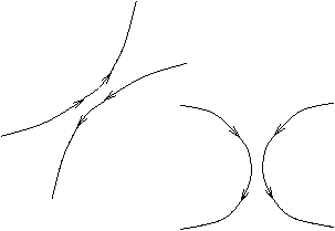
Figure 7.1 - Impossible to Distinguish between Different Particles
In quantum theory fundemental particles are indistinguishable.
Þ |Y (1,2)|2=|Y (2,1)|2
more generally
| Y (1,2)=e |
|
Y (2,1)=e |
|
Y (1,2) |
Y (1,2)=±Y (2,1)
so there are two possible outcomes of this
Y (1,2)=Y (2,1) (7.2)
this (the class is called Bosons) obeys Bose-Einstein Statistics whilst
Y (1,2)=-Y (2,1) (7.3)
obeys Fermi-Dirac Statistics (the class of particles here are called Fermions).
7.2.1 Spin - Statistics Theorem
Particles of 1/2 integer spin are fermons (electrons, protons, neutrons, He3 , ...). Particles of integer spin are bosons (photons, gravitons, W, Z, Higgs, He4 , ...). The He3/4 are made up of other combinations of spin (the proof is in the Atomic Physics's Module).
Points to take note about
-
generally for fermions and bosons, permultations don't change the physical state
- in addition for fermions
Y (1,2)=-Y (2,1)
therefore Y =0 if " 1=2 ", ie if both are in the same state. This is the Pauli Exclusion Principle.
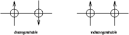
Figure 7.2 - Situations Where We Can Distinguish the Difference
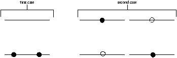
Figure 7.3 - Counting For Two Levels - What is
W ?
For the first case in a classical view W=1 , for the Bose-Einstein case W=1 and for the Fermi-Dirac case W=0 . For the second case in a classical view W=2 , Bose-Einstein its W=1 and the Fermi-Dirac states W=1 .
7.3 Equilibrium Occupation Numbers
7.3.1 The Bose-Einstein Case
we assume that gSnS>>1 and we maximise so that S=klnW is subjected to åSnS=N and åSnSeS=U .
we now consider
we now set df=0 and we obtain the equilibrium values of nS
| f= |
|
[ |
(gSnS)ln(gS+nS)-gS-nS-nSlnnS+nS-ln(gS!) |
] |
+a |
|
nS-b |
|
eSnS |
| df= |
|
[ |
ln(gS+nS)-lnnS+a-b eS |
] |
dnS |
7.3.2 The Fermi-Dirac Case
7.3.3 The Classical Case (Limit)
7.3.4 Interpretations of the Constants
Both a and b are determined by
however in general this is a difficult approach and also we don't introduce a partition function Z .
Instead we consider the condition for S=klnW to be maximised so that
this means that
dS+ka dN-kb dU=0 (at fixed eS)
we now compare this to
dU=TdS-PdV+µ dN
however PdV=0 as eS is a constant
we can now rewrite the following
where there is a minus in the Bose-Einstein case and a plus in the Fermi-Dirac case.
7.4 Fermi-Dirac Gases
As nS approaches gS then the quantum effects start becoming important. The applications of this are
-
electrons in metals
- 3He at low temperatures
- neutron and white dwarf stars
so f(e )=0 if e >µ , f(e )=1/2 if e =µ and f(e )=1 if e <µ .
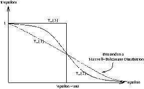
Figure 7.4 - Plotting the Three Different States of Positioning
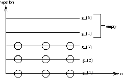
Figure 7.5 - Fermion's Dropping into the Lowest States
e=e (U); µ =µ (T,V)
The properties of f(e ) depend on µ as
f(e )=1 when e <µ f(e )=0 when e >µ (7.8)
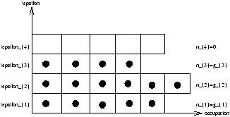
Figure 7.6 - The Fermi-Dirac Ground State
As T® 0 , each particle drops into the lowest possible state, however the exclusion princliple prevents occupation with nS>gS , so each level fills to the maximum nS=gS , then the next energy level fills up to a maximum energy level e =µ . So µ is the energy of the highest occupied state and nS=0 for eS>µ . µ in this context is also called eF which is known as the Fermi Energy.
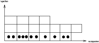
Figure 7.7 - The Bose-Einstein Ground State
7.4.1 The Calculation of mu (epsilon-F)
Now refering back to equation 7.8 we can obtain
where g(e ) is the degeneracy (from equation 6.25).
In the case of electrons the value of g(e ) has a multiple of two added as an electron can also have two different states of spin.
This equation can be used to calculate µ in terms of N
We define the Fermi temperature by µ =kTF
The Fermi-Dirac effects are important for when T<<TF . For example, electrons in a metal TF~ 70,000K . So Fermi-Dirac statistics are important at room temperature.
where l is the thermal de Broglie wavelength (looked at in section 7.1)
| Þ |
|
~ |
æ
ç
ç
ç
ç
ç
è |
|
ö
÷
÷
÷
÷
÷
ø |
|
=(e |
|
) |
|
Internal Energy
| U= |
|
nSeS~ó
õ |
de f(e )g(e )e = |
ó
õ |
|
de g(e )e =2C× |
ó
õ |
|
dee |
|
|
Þ U= |
|
µ N= |
|
NkTF (at T=0) (7.11) |
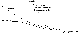
Figure 7.8 - The Exclusion Principle
note that
7.5 Bose-Einstein Condensation
The properties of fS depend on µ (T,V) as T® 0 by using åSnS£ N . As T® 0 we expect all the particles to drop into the lowest energy state s=0 , energy e0 and degeneracy g0=1 .
Þ n0® 0 as T® 0
Þ n1® 0
Þ n2® 0
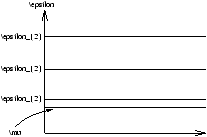
Figure 7.9 - Seperation of Energy Levels
Generally we have
|e0-µ |<<|e1-e0|
for example
If m=He4 , m~ 7× 10-27kg , ~ 10-34Js , we now let L=1cm so that
e~ 10-35J
| µ~ - |
|
, T~ 1K, K~ 10-23JK-1, N~ 1023 |
Þ µ~ -10-46J
this is very small
where in the n0 equation µ is very small whilst in the n1 equation it is not very small, ie. the particles drop into n0 extremely rapidly as T® 0 .
If we compare this to the classical case
For Bose-Einstein Statistics
and because e-µ/kT~ 1+1/N we obtain
| Þ |
|
~ 1023× 10-12~ 1011>>1 at T=1K |
note that
7.6 Photons and Blackbody Radiation
We have seen that
we now consider radiation in a cavity where the energy level is related to the frequency ( e =hn , degeneracy g(e ) ), we compute U
to fix a we use åSnS=N however photons are not conserved in number. This implies that a is zero because this is the Lagrange multiplier for åSnS=N .
what is g(e ) ?
and this becomes
this is known as Planck's Radiation Law
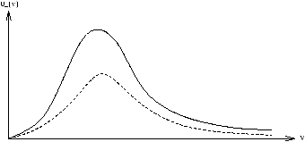
Figure 7.10 - Blackbody Radiation Plot
let x=hn/kT , n=kT/hx
where
and
this is known as Stefan-Boltzmann Radiation Law