


Chapter 4 The Fundemental Law
4.1 Combined First and Second Laws
dU=d-6mu'26 Q-d-6mu'26 W
d-6mu'26£ TdS
or for a reversible process
d-6mu'26 =TdS
d-6mu'26 W£ PdV
or for a reversible process
d-6mu'26 W=PdV
For reversible processes we therefore have
dU=TdS-PdV (4.1)
This is the fundamental equation of thermodynamics
However this equation now depends on state functions only (so there is no Q or W ). It describes the relationship between state variables at neighbouring equilibrium points. So it is independent of whether we move between those points by a reversible or irreversible process.
4.2 Mathematical Structure
dU=TdS-PdV
U=U(S,V)
| Þ dU= |
æ
ç
ç
è |
|
ö
÷
÷
ø |
|
dS+ |
æ
ç
ç
è |
|
ö
÷
÷
ø |
|
dV |
| T= |
æ
ç
ç
è |
|
ö
÷
÷
ø |
|
, P=- |
æ
ç
ç
è |
|
ö
÷
÷
ø |
|
| |
æ
ç
ç
è |
|
ö
÷
÷
ø |
= |
|
= |
|
=- |
æ
ç
ç
è |
|
ö
÷
÷
ø |
|
|
|
æ
ç
ç
è |
|
ö
÷
÷
ø |
=- |
æ
ç
ç
è |
|
ö
÷
÷
ø |
|
(4.2) |
4.2.1 An Example
S=S(U,V)
| |
æ
ç
ç
è |
|
ö
÷
÷
ø |
|
= |
|
, |
æ
ç
ç
è |
|
ö
÷
÷
ø |
|
= |
|
4.3 Internal Energy
Given the equation of state (eg. Van der Waal's) what can we say about U(T,V)?
dU=TdS-PdV
we want U=U(T,V) so let S=S(T,V)
| Þ dS= |
æ
ç
ç
è |
|
ö
÷
÷
ø |
|
dT+ |
æ
ç
ç
è |
|
ö
÷
÷
ø |
|
dV |
| dU=T |
æ
ç
ç
è |
|
ö
÷
÷
ø |
|
dT+ |
é
ê
ê
ê
ê
ê
ë |
T |
æ
ç
ç
è |
|
ö
÷
÷
ø |
|
-P |
ù
ú
ú
ú
ú
ú
û |
dV |
| dU= |
æ
ç
ç
è |
|
ö
÷
÷
ø |
|
dT+ |
æ
ç
ç
è |
|
ö
÷
÷
ø |
|
dV |
|
|
æ
ç
ç
è |
|
ö
÷
÷
ø |
|
=T |
æ
ç
ç
è |
|
ö
÷
÷
ø |
|
(4.3) |
|
|
æ
ç
ç
è |
|
ö
÷
÷
ø |
|
=T |
æ
ç
ç
è |
|
ö
÷
÷
ø |
|
-P (4.4) |
| |
|
(equation 4.3)= |
|
(equation 4.4) |
| T |
|
= |
æ
ç
ç
è |
|
ö
÷
÷
ø |
|
+T |
|
- |
æ
ç
ç
è |
|
ö
÷
÷
ø |
|
|
|
æ
ç
ç
è |
|
ö
÷
÷
ø |
|
=T |
æ
ç
ç
è |
|
ö
÷
÷
ø |
|
-P (4.5) |
4.3.1 An Ideal Gas
P=NkT/V so equation 4.5 gives
therefore as expected U=U(T) .
4.3.2 A Van der Waals Gas
now we insert into equation 4.5
| |
æ
ç
ç
è |
|
ö
÷
÷
ø |
|
=T |
|
-P=P+a |
|
-P (using the equation of state) |
4.3.3 An Application - Temperature Change in Free Expansion
V0® V1 in adiabatic free expansion and so there is no work done ( W ) or heat flow ( Q ) so
D U=0
however T may drop for a Van der Waal's gas.
Let T=T(V,U)
| dT= |
æ
ç
ç
è |
|
ö
÷
÷
ø |
|
dV+ |
æ
ç
ç
è |
|
ö
÷
÷
ø |
|
dU |
| µJ= |
æ
ç
ç
è |
|
ö
÷
÷
ø |
|
=Joule Coefficient |
| |
æ
ç
ç
è |
|
ö
÷
÷
ø |
|
æ
ç
ç
è |
|
ö
÷
÷
ø |
|
æ
ç
ç
è |
|
ö
÷
÷
ø |
|
=-1 |
| |
æ
ç
ç
è |
|
ö
÷
÷
ø |
|
=- |
æ
ç
ç
è |
|
ö
÷
÷
ø |
|
æ
ç
ç
è |
|
ö
÷
÷
ø |
|
=- |
|
æ
ç
ç
è |
|
ö
÷
÷
ø |
|
(cvdT=d-6mu'26 QV=dU)
or from using the energy equation we obtain
| |
æ
ç
ç
è |
|
ö
÷
÷
ø |
|
=- |
|
é
ê
ê
ê
ê
ê
ë |
T |
æ
ç
ç
è |
|
ö
÷
÷
ø |
|
-P |
ù
ú
ú
ú
ú
ú
û |
4.4 Entropy from the Fundamental Equation
The Fundamental Equation when rearranged says
so if we know U and P we may get S=S(T,V) . For an ideal gas U=3/2kT for the monotomic case and PV=NkT . We plug these values in an obtain
| Þ S= |
|
NklnT+NklnV+constant |
For the case of a Van der Waal's gas where U=3/2NkT-aN2/V
| dS= |
|
æ
ç
ç
è |
|
NkdT+a |
|
dV |
ö
÷
÷
ø |
+ |
|
dV |
The Entropy (in ??TD??) has no absolute meaning but we can compare entropy changes in Van der Waal's and the Ideal cases.
| (D S)Van der Waals-(D S)ideal=Nkln |
|
-Nkln |
|
| (D S)Van der Waals-(D S)ideal=Nkln |
|
(D S)Van der Waals>(D S)ideal (if V>V0)
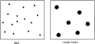
Figure 4.1 - Comparing the Ideal and Van der Waal Case
In the Van der Waal case the molcules occupy a finite volume b whilst in the ideal case the molecules are points. So in an expansion the molecules in the Van der Waal case experience a greater increase in freedom relative to the ideal case.
Þ (D S)Van der Waals>(D S)ideal
4.5 Entropy Max Principle
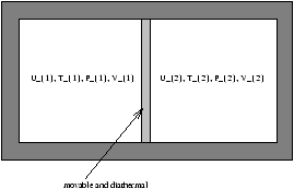
Figure 4.2 - ?????An Experiment?????
What are the equilibrium conditions? We use the Entropy Max Principle:
S=S1+S2 is maximized at equilibrium, subject to fixed U=U1+U2 and V=V1+V2 .
Therefore S is a maximum when dS=0
Þ dS1=-dS2
so when
dU=0Þ dU1=-dU2
dV=0Þ dV1=-dV2
so now the equilibrium condition is
so U1 and V1 are independent variables
T1=T2, P1=P2
so the Entropy Max Principle and the Fundamental Equation of ??TD?? gives us the equilibrium conditions.
4.6 Paramagnetism
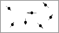
Figure 4.3 - A Box Full of Fixed Particles Each of Which is a Small Magnet
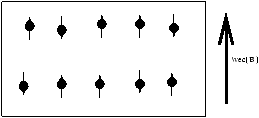
Figure 4.4 - The Box of Magnets Placed in a Magnetic Field
In the presence of a magnetic field the dipoles either align parallel or anti parallel to the magnetic field.
N=n1+n2 dipoles
where n1 is the number of dipoles aligned with B ( e1=-mB ) and n2 is the number of dipoles counter aligned with B ( e2=+mB ).
The total magnetism is
M=m(n1+n2) (M=Nm at t=0)
Total Energy is
U=n1(-mB)+n2(+mB)
® U=-(n1-n2)mB=-MB
The Fundemental Equation (from Electricity and Magnetism first year)
dU=TdS-MdB
as M is extensive and B is intensive this means that B is like -P and M is like V . This is analogous to
d(U+PV)[=H]=TdS+VdP
so U=-MB is analogous to enthalpy H .
We also now need an equation of state
for some constant c at high temperatures.
From this we can tell that the isotherms are Mµ B and the adiabats are
dU=0-MdB
-d(UB)=-MdB
-dM.B-MdB=-MdB
Þ M=constant
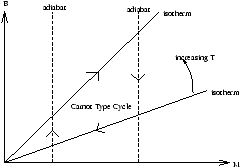
Figure 4.5 - Isotherms and Adiabats in Magnetism
4.6.1 Entropy
| Þ dS- |
|
dM=- |
|
dM (by Curie's Law) |
We can also derive the energy equation
| Þ |
æ
ç
ç
è |
|
ö
÷
÷
ø |
|
=T |
æ
ç
ç
è |
|
ö
÷
÷
ø |
|
-M |
4.7 A Preview of Statistical Mechanics
In Statistical Mechanics we look at the statistics of energy levels to get Thermodynamic information.
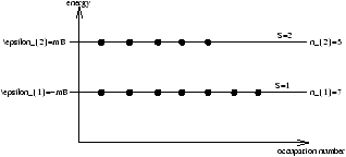
Figure 4.6 - The Model Used in Statistical Mechanics
What are the values of n1 and n2 at equilibrium at a temperature T ?
Statistical Mechanics tells us that the probability of being in level S is proportional to the Boltzmann Distribution.
for some constant Z , to fix Z we use
so we obtain Z=å e-eS/kT normalises the function, Z is called the Partition Function; so
we now compute M and the equation of state becomes
M=m(n1-n2)
Thus the equation of state is
tanhx~ x (for small x)
ie. this is as for Curie's Law (for high T ).
The values of n1 and n2 as T® 0 and T®¥
as T® 0 Þ n1® 1 and n2® 0
so as T®¥ ( kT>>mB ) there is an equal probability of the occupation of 1 or 2. However as T® 0 n1® N and n2® 0 , meaning that the highest probability is in the lowest state.