


Chapter 2 The First Law
2.1 Simple Processes
Quasistatic (QS) processes are so slow that they are a series of equilibrium states. If there are large departures from equilibrium we call it non-static.
Important QS processes:
-
Isothermal:
- constant temperature experiment. This is usually done by maintaining contact with a reservoir (eg. ice bath).
- Adiabatic:
- there is no heat flow in the experiment across boundaries.
- Isobaric:
- constant pressure experiment.
- Isochoric:
- constant volume experiment.
Equilibrium states and QS processes may be plotted on an indicator diagram (otherwise know as a P against V diagram (or PV diagram)).
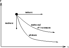
Figure 2.1 - an Indicator (
PV ) Diagram
Non-static processes may not be represented on a PV diagram although the end points can be, if they are equilibrium states.
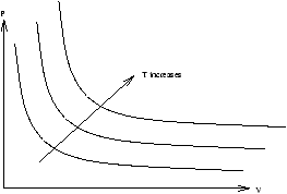
Figure 2.2 -
PV plot of Isotherms
2.2 Work
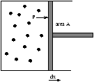
Figure 2.3 - Work Done By A Gas
work done by a gas is
W=F× dx=PAdx=PdV<0
For finite changes V1® V2 and so the work done by a gas is
2.2.1 An Example
QS isothermal expansion of an ideal gas
PV=NkT=constant
| W= |
ó
õ |
|
PdV=NkT |
ó
õ |
|
|
=NkT[ln V |
] |
|
=NkT |
( |
ln V2-ln V1 |
) |
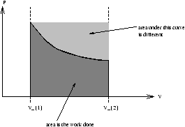
Figure 2.4 -
PV Diagram of Work Being Done
| W= |
ó
õ PdV=area under curve |
òV1V2PdV depends on the curve from P1V1® P2V2 , ie. work done depends on the process (work is not a function of state).
Therefore we write
PdV=d-6mu'26 W
This d-6mu'26 W is an inexact differential, therefore òd-6mu'26 W depends on the path.
For an exact differential ( df ) ò df depends only on the end-points and not on the path.
2.2.2 Exact and Inexact Differentials
Any object of the form u(x,y)dx+v(x,y)dy is called a differential.
-
if udx+vdy=df , for some function f(x,y) , then the differential is exact
| |
ó
õ |
(udx+vdy)= |
ó
õ df=[f]end points |
- if udx+vdy¹ df for any f , then the intergral ò (udx+vdy) depends on the path and so the differential is inexact.
An Exact Differential Example
| |
ó
õ |
|
(xdx+ydy)= |
ó
õ |
|
d |
æ
ç
ç
è |
|
x2+ |
|
y2 |
ö
÷
÷
ø |
= |
é
ê
ê
ë |
|
x2+ |
|
y2 |
ù
ú
ú
û |
|
An Inexact Differential Example
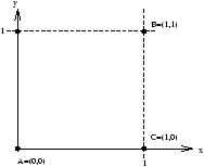
Figure 2.5 - An Inexact Differential
Along the path AB
| |
ó
õ |
|
(ydx+xdy)= |
ó
õ |
|
(xdx-xdx)=0 |
| |
ó
õ |
|
(ydx-xdy)= |
ó
õ |
|
ydx- |
ó
õ |
|
xdy=0- |
ó
õ |
|
dy=-1 |
2.2.3 Back to Work Examples
a gas
dW=PdV
an extensible wire
d-6mu'26 W=F dx (2.3)
where F is the tension the wire
a charge q in an electric field
d-6mu'26 W=qE.dr (2.4)
2.3 First Law
Work depends on the process because the different paths draw in different amounts of heat. So let us concentrate on adiabatic work (not heat flow). Then we find the work done is the same for all processes.
This implies the first law of thermodynamics (in its first form):
-
First Law of Thermodynamics:
- For every adiabatic process between two equilibrium states, work done is the same (they don't need to be QS).
This first law implies that adiabatic work ( Wad ) is represented by an exact differential ( dWad ) (because it is path independent).
let dWad=-dU (2.5)
Wad=-(U2-U1)
U is a new function of state - internal energy.
you may take U as being U(T,V) , U(T,P) or U(T,V) . If U=U(T,V)
| dU= |
æ
ç
ç
è |
|
ö
÷
÷
ø |
|
dT+ |
æ
ç
ç
è |
|
ö
÷
÷
ø |
|
dV |
| dU= |
æ
ç
ç
è |
|
ö
÷
÷
ø |
|
dT+ |
æ
ç
ç
è |
|
ö
÷
÷
ø |
|
dP |
Now we extend to include heat. Suppose we go between two equilibrium states by two routes
-
adiabatically
- non-adiabatically (heat flows)
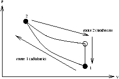
Figure 2.5 - Heat Flowing on a
PV Diagram
In both cases U1® U2 (since U is a function of state). In route 1 U2-U1=-Wad (from the first law). In route 2 a different amount of work W is done as heat flows U1® U2 .
We define heat by
Q=W-Wad (2.6)
Q=W+U2-U1
U2-U1=Q-W (2.7)
Equivalently
dU=d-6mu'26 Q-d-6mu'26 W (2.8)
This is the first law in its differential form, notice that its of the form (exact)=(inexact)+(inexact) .
2.3.1 New Ideas
-
existence of U
- conservation of energy
- definition of heat
2.3.2 Conservation of Heat
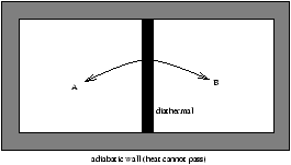
Figure 2.6 - The Conservation of Heat
D UA=QA-WA, D UB=QB-WB
D (UA+UB)=QA+QB-(WA+WB)
where D (UA+UB) is the D U for the whole system and (WA+WB) is the work for the whole system.
as there are adiabatic walls we get instead
D (UA+UB=-(WA+WB)
QA=-QB (2.9)
so we can say heat lost by B equals the heat gained by A.
2.4 Internal Energy of An Ideal Gas
We need more information on U(T,V)
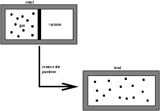
Figure 2.7 - Joule's Experiment of Free Expansion
Joule found that for an ideal gas under free expansion
-
Tinitial=Tfinal (2.10)
- the first law says
Uinitial=Ufinal
ie.
U(Tinitial,Vinitial)=U(Tfinal,Vfinal)
U(T,Vinitial)=U(T,Vfinal)
because Tinitial=Tfinal=T say
| Þ |
æ
ç
ç
è |
|
ö
÷
÷
ø |
|
=0 (for an ideal gas) |
U=U(T) (2.11)
- another consquence of Joule's experiment
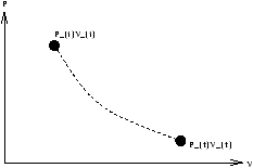
Figure 2.8 -
PinitialVinitial=
PfinalVfinal
But the process between is a non-static process ( P , T , ... are non-uniform and time dependent). So this inbetween region cannot be plotted on a PV diagram, however Joule's experiment implies that Tinitial=Tfinal so the end-points lie on an isotherm.
An ideal gas is often defined by PV=NkT and U=U(T) . To get further information on U(T) we need the specific heats.
For example the specific heat at constant pressure
For example the specific heat at constant volume
CV is the ratio of the differentials (because Q is not a state function).
2.4.1 specific heat at constant volume
dU-d-6mu'26 Q-d-6mu'26 W=d-6mu'26 Q-PdV
d-6mu'26 Q=dU+PdV
|
Cv= |
æ
ç
ç
è |
|
ö
÷
÷
ø |
|
= |
æ
ç
ç
è |
|
ö
÷
÷
ø |
|
(2.14) |
| Cv= |
|
(T) (for an ideal gas) |
d-6mu'26 Q=dU+PdV=CvdT+PdV (for an ideal gas)
2.4.2 specific heat at constant pressure
| Cp= |
æ
ç
ç
è |
|
ö
÷
÷
ø |
=Cv+P |
æ
ç
ç
è |
|
ö
÷
÷
ø |
|
PV=NkT (for an ideal gas)
Cp=Cv+Nk (for an ideal gas) (2.15)
Cp and Cv may depend on T , P , etc. Experimentally, for all ideal gases
-
Cp , Cv are functions of T only
- for monotomic gases
- for diatomic
We can now introduce the g factor.
Going back to U(T)
U(T)=CvT+constant
|
U(T) (monotomic)= |
|
NkT U(T) (diatomic)= |
|
NkT (2.16) |
f=3 (for monotomic® three translational)
f=5 (for diatomic® three translational, two rotational)
At high temperatures ( T ) there can be two more degrees of freedom, these come from the vibrational modes of the molecules.
2.5 Equation of an Adiabat
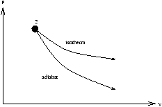
Figure 2.8 -
PV Isoterm Reminder
For adiabatic expansion d-6mu'26 Q=0
dU=d-6mu'26 Q-PdV=-PdV
U=CvT, PV=NkT
however Nk/Cv=g -1
By re-expressing in P and V
substitute in equation 2.20
2.6 Enthalpy
| Cv= |
æ
ç
ç
è |
|
ö
÷
÷
ø |
|
= |
|
(function of state) |
| Cp= |
æ
ç
ç
è |
|
ö
÷
÷
ø |
|
= |
|
( |
? |
) |
(can we find the '?') |
dU=d-6mu'26 Q-PdV=d-6mu'26 Q-d(PV) (if P=constant)
d-6mu'26 Q=d(U+PV)
we define Enthalpy as
H=U+PV (2.20)
Now d-6mu'26 Q=dH at constant P therefore
2.7 Some Mathematical Results - See Handout