


Chapter 26 Lecture 25 - Examples of Perturbation Theory
26.1 Non-Degenerate Perturbation Theory
We recall from the last lecture that
En~ En0+D En(1)+D En(2) (26.1)
We will now apply these results to study the behaviour of a distorted infinite square well.
V=¥ , x<0, x>L Þ V'=Cx(x-L) (0<x<L) (26.3)
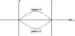
Figure 25.1 - A Distorted Infinite Square Well
H0 is the potential of the infinite square well
V'=Cx(x-L) (where lº C) (26.4)
we now assume that l (C) is sufficiently small and now we obtain
The first order energy shift is
| D En(1)=l |
ó
õ |
|
Un*(x)VUn(x)dx |
| D En(1)=C |
ó
õ |
|
Un*(x)x(x-L)Un(x)dx |
|
Þ D En(1)=-CL2 |
æ
ç
ç
è |
|
+ |
|
ö
÷
÷
ø |
(26.6) |
|
En= |
|
-CL2 |
æ
ç
ç
è |
|
+ |
|
ö
÷
÷
ø |
(26.7) |
The changes to the wavefunction mean that we must evalute Ck(1)
note that if k+n is odd then this integral vanishes as ck(1)=0 however if k+n is even the the integral is finite and becomes
If n=1 in this case (eg. the ground state) the contribution to ck(1) is only from when k is odd.
26.1.1 Example - Nuclear Square Well
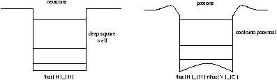
Figure 25.2 - The Nuclear Square Well
The outcomes of this model are
-
the states of the protons are shifted up in energy
- th protons wavefunction is localised closer to the walls
26.2 Degenerate Perturbation Theory - A Hydrogen Atom in an Electric Field
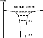
Figure 25.3 - A Hydrogen Atom in an Electric Field
The energy states are characterised by the priniciple quantum number n , where each value of n has l=n-1,n-2,... ,0 . In a Hydrogen atom the n=2 state has properties
| n=2 state |
Four Fold Degeneracy |
| l=0 |
1 |
| m=0 |
1,0,-1 |
| |
we write Un,l,m , so for n=2 we have U2,0,0 , U2,1,1 , U2,1,0 and U2,0,-1 all with the same energy E20 .
The electric field F is now applied along the z direction.
Now the interaction along the Hamiltonian Vinternal=ezF and so
H=H0+ezF (26.10)
we obtain that V'=ezF so the new eigenstates of the problem are
f1=U2,1,0+U2,0,0 f2=U2,1,0-U2,0,0 f3=U2,1,1 f4=U2,1,-1 (26.11)
we recall from the handout that
D E3(1)=D E4(1)=0 (26.12)
| D E1,2= |
ó
õ |
|
ó
õ |
|
ó
õ |
|
f1,2*(r)ezFf1,2(r)r2sinqdrdq df |
D E1,2=± 3eFa0 (26.13)
this is known as the Stark effect.