Chapter 27 Lecture 26 - Systems With Several Particles

27.1 Multiple Particle Wavefunctions

For a single particle we can define a wavefunction Y (r) which when manipulated to |Y (r)|² which can be interpreted as a probility density.

For a N-particle system the wavefunction becomes

Y (r₁,r₂,... ,r_N) (27.1)

so that |Y (r₁,r₂,... ,r_N)|² can be interpreted as a joint probability, ie the probability that a particle one is at position r₁ , that particle two is at position r₂ , etc.

The N-particle Schrödinger equation

HY (r₁,r₂,... ,r_N)=EY (r₁,r₂,... ,r_N) (27.2)

H is an N-particle Hamiltonian composed of

N kinetic energy operators, ie -²/2m₁Ñ₁² , ...
N single particle potentials, ie V₁(r₁) , ...
interaction potentials between pairs of particles
V_1,2(r₁,r₂), ... ,V_1,N(r₁,r_N)

27.2 Non-Interacting Particles

In this case if there is no interaction then we obtain a simplifed version of the Hamiltonian

k=1

æ
ç
ç
è

2m_k

Ñ_k²+V_k(r_k)

ö
÷
÷
ø

(27.3)

H is the sum of N independent particle Hamiltonians.

Y (r₁,r₂,... ,r_N)=U⁽¹⁾(r₁)U⁽²⁾(r₂),... ,U^(N)(r_N) (27.4)

where U^(k) is the state of the k'th particle and r_k is the position coordinate of the k'th particle.

In this case

HY (r₁,r₂,... ,r_N)=

æ
ç
ç
è

k=1

E^(k)

ö
÷
÷
ø

Y (r₁,r₂,... ,r_N) (27.5)

This is useful because

often we can ignore particle interactions
if there is an interaction, eg.

V_i,kµ

1

|r₁-r_k|

then with equations V.64 and V.65 we obtain zero order solutions

27.3 Identical Particles

The could be for example pairs of electrons, protons, neutrons or a particles. When in the same energy and spin states such that they are fundementally indistinguishable.

To investigate this we will consider a generic elastic scattering experiment between two particles, which we will label 1 and 2 (but these may be identical). We will be working the the centre of mass frame

Figure 26.1 - The Centre of Mass Frame

f₁(q ) is the scattering probability amplitude for the particle i to be scattered into the angle q .

We place the detectors DI and DII at locations q and (p -q )

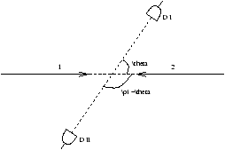
Figure 26.2 - The Scattering Experiment

There are two ways to register hits simultanously at DI and DII

case A:: forward scattering

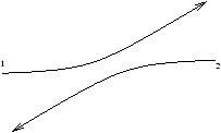
Figure 26.3 - Forward Scattering Result

probability detection 1 at DIµ |f_A,1(q )|² probability detection 2 at DIIµ |f_A,2(p -q )|² (27.6)
by conservation of momentum
|f_A,2(p -q )|²=|f_A,1(q )|²
case B:: backward scattering

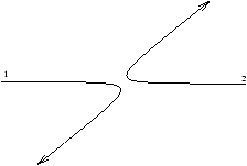
Figure 26.4 - Backward Scattering Result

probability detection 1 at DIIµ |f_B,1(p -q )|² probability detection 2 at DIµ |f_B,2(q )|² (27.7)
by conservation of momentum
|f_B,1(p -q )|²=|f_B,2(q )|²

Now since both case A and B can occur how do the probabilities of these events combine? What is the total probability of the detector DI seeing particles?

If q =p/2 we should find by symmetry

½
½
½
½

f_A,1

æ
ç
ç
è

ö
÷
÷
ø

½
½
½
½

f_B,2

æ
ç
ç
è

ö
÷
÷
ø

½
½
½
½

æ
ç
ç
è

ö
÷
÷
ø

½
½
½
½

(27.8)

Summarising experimental results

spin	particle 1	particle 2	q=p/2	q
0	a	p	2\|f(p/2) \|²	\|f_A(q )\|²+\|f_B(p -q )\|²
0	a	a	4\|f(p/2) \|²	\|f_A(q )+f_B(p -q )\|²
1/2	p	p¯	2\|f(p/2) \|²	\|f_A(q )\|²+\|f_B(p -q )\|²
1/2	p	p	0	\|f_A(q )-f_B(p -q )\|²

so for non-identical particles we add the probabilities however for identical particles we add the amplitudes.

There are two types of particles, ones with spin 0 - where we get constructive interference (bosons) and half spin where we get destructive interference (fermions).