Chapter 25 Lecture 24 - Perturbation Theory

25.1 The Quantum Mechanics of Real Systems

We can find exact analytical solutions to

the infinite square well
the harmonic oscillator ( V(x)µ x² )
the comlomb potential ( V(x)µ -1/r )

However these are more or less the only analytical solutions we can obtain.

Although main systems can be approximated to the three analytical solutions we still need to be able to call upon procedures to obtain more accurate solutions to real systems. We can solve these problems through one of two methods

use a numerical integration of Schrödinger's Equation (via the use of supercomputers)
use a systematic approximation method, this is whats called Perturbation Theory

H=H₀+V' (25.1)

H₀ is exactly soluble giving us the zero order solutions whilst V' is a small perturbation. For example

H=-

d²

dx²

+a x²+b x³

where H₀ is represented by -²/2md²/dx²+a x² (this is where the real system can be approximated to a hormonic oscillator) and V' is represented by b x³ .

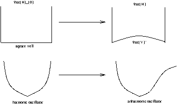
Figure 24.1 - Application of Perturbation Theory to a Real System

25.2 Perturbation Theory

Solutions to H are built iteratively from solutions to H₀ . This is sensible since the eigenstates of H₀ form a complete set.

H₀U_n=E_n⁰U_n (25.2)

we now say that each eigenvalue E_n⁰ is associated with a single state U_n (non-digenerate).

We will now write

V'=lH(r) (25.3)

where V(r) is a form of the potential that has been normalised whilst l is the strength of interaction (the scaling factor).

H=H₀+lV(r) (25.4)

our procedure works best if l is very small.

D E

E_n⁰

<<1

The eigenstates of H are labeled Y_n and the eigenvalues of H are labeled E_n .

Formally we can write these as a power series in l

Y_n=Y_n⁽⁰⁾+lY_n⁽¹⁾+l²Y_n⁽²⁾+... (25.5)

E_n=E_n⁽⁰⁾+l E_n⁽¹⁾+l²E_n⁽²⁾+... (25.6)

since l<<1 there rapidly converge. The zero order solutions can be equated to the unperturbed system

Y_n⁽⁰⁾=U_n E_n⁽⁰⁾=E_n⁽⁰⁾ (25.7)

Schrödinger's Equation

HY_n=E_nY_n

(

H₀+l V(r)

)

[

F_n⁽⁰⁾+lY_n⁽¹⁾+l²Y_n⁽²⁾+...

]

[

E_n⁽⁰⁾+l E_n⁽¹⁾+l²E_n⁽²⁾+...

]

[

Y_n⁽⁰⁾+lY_n⁽¹⁾+Y_n⁽²⁾+...

]

(25.8)

The terms of the same order of l can be collected and equated thus

order lÞ V(r)U_n+H₀Y_n⁽¹⁾=E_n⁽¹⁾U_n+E_n⁰Y_n⁽¹⁾ (25.9)

order l²ÞV(r)Y_n⁽¹⁾+H₀Y_n⁽²⁾=E_n⁽²⁾U_n+E_n⁽¹⁾Y_n⁽¹⁾+E_n⁰Y_n⁽²⁾ (25.10)

To proceed Y_n⁽¹⁾ (or Y_n⁽²⁾ ) can be expanded in terms of the eigenstates of H₀

Y_n⁽¹⁾=

k n

c_k⁽¹⁾U_k (25.11)

If this is substituted into equation V.38 and we apply the procedure for using orthogonality to elimate most of the terms ò_all spaceU_j^*dV we obtain for j=n the first order energy shift

D E_n⁽¹⁾=l E_n⁽¹⁾=l

ó
õ

all space

U_n^*(r)V(r)U_n(r)dV=l <n|V|n> (25.12)

this is just the expectation value of V . However if j n we obtain c_j⁽¹⁾ first order correction to the expansion coefficient

c_j⁽¹⁾=l

ó
õ

all space

U_j^*VU_ndV

E_n⁰-E_j⁰

(25.13)

For the second order energy shifts

D E_n⁽²⁾=l²

k n

ó
õ

all space

U_k^*VU_ndV|²

E_n⁰-E_n⁰

(25.14)

E_n~ E_n⁰+D E_n⁽¹⁾+D_n⁽²⁾ (25.15)