Chapter 18 Lecture 17 - Three Dimensional Systems

18.1 Introduction

If we go beyond one dimension the basic rules of Quantum Mechanics are unchanged. The only implications are that

we have to be aware of the geometry and symmetry of our system and choose an appropriate coordinate system to work in
in three dimensions we have also to consider angular momentum

18.2 Three Dimensional Hamiltonian

Schrödinger's Equation in one dimension is

é
ê
ê
ë

d²

dx²

+V(x)

ù
ú
ú
û

Y (x)=EY (x)

however in three dimensions it becomes

é
ê
ê
ë

Ñ²+V(r)

ù
ú
ú
û

Y (r)=EY (r) (18.1)

H is in terms of Ñ² and V(r) . So in Cartesian Coordinates

Ñ²=

¶²

¶ x²

¶²

¶ y²

¶²

¶ z²

(18.2)

and

V(r)=V(x,y,z)

Y (r)=Y (x,y,z)

This is convienent if the basic geometry is compatible (eg. a crystal lattice). Often it is more appropiate to work with spherical coordinates. For example in atoms and nuclei as there is a central symmetry.

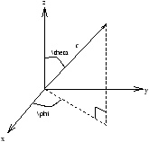
Figure 17.1 - The Spherical Coordinate System

In spherical polars we have

Ñ²=

¶²

¶ r²

¶ r

r²

æ
ç
ç
è

¶²

¶q²

+cotq

¶q

sin²q

¶²

¶f²

ö
÷
÷
ø

(18.3)

where the radial part is made up with ¶²/¶ r²+2/r¶/¶ r and the angular part is 1/r²(¶²/¶q²+cotq¶/¶q+1/sin²q¶²/¶f²) .

V(r)=V(r,q ,f )

Y (r)=Y (r,q ,f )

So to integrate (in the form ò_all space[<integrand>]dV ) over the volume:

cartesian:

ó
õ

-¥

ó
õ

-¥

ó
õ

-¥

[ ]dxdydz (18.4)

spherical polar:

ó
õ

[ ]r²sinqdq df dr (18.5)

this is because 0£ r£¥ , 0£f£ 2p and 0£q£p .

18.2.1 Example - Normalisation of a Three Dimensional Wavefunction

The S-State of Hydrogen is

f (r)=e

r₀

|c|²=

ó
õ

r₀

r²sinqdq df dr=1

the e^-^2r/r_⁰^r^² is obtained from Y^*Y

p r₀³

18.3 Parity

Symmetry considerations give an important insight, this helps us with

boundary conditions
compatibility of measurements

We define a parity transformation associated with the parity operator ( P )

PY (x,y,z)=Y (-x,-y,-z) (18.6)

If the system has a well defined parity (definate parity) then

PY (x,y,z)=±Y (x,y,z) (18.7)

however the parity transformation in spherical coordinates is

PY (r,q ,f )=Y (r,p -q ,f +p ) (18.8)

On the compatibility of these operators

[P,p²]=0 compatible (18.9)

in a central potential

[P,H]=0 (18.10)

ie. in a symmetric potential, eigenstates of energy are also eigenstates of parity

18.4 Angular Momentum

In addition to linear momentum there is now a (rotational) angular momentum

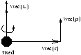
Figure 17.2 - Angular Momentum

In a central potential angular momentum is conserved (both classically and quantum mechanically)

L=r×p (18.11)

In cartesian coordinates

½
½
½
½
½

i	j	k
x	y	z
p_x	p_y	p_z

½
½
½
½
½

=il_x+jl_y+kl_z (18.12)

where

l_x=yp_z-zp_y l_y=xp_z-zp_x l_z=xp_y-yp_x (18.13)

so we can define a quantity that is the total angular momentum

|L|²=l_x²+l_y²+l_z² (18.14)