


|
æ ç ç è |
A | A+ |
|
ö ÷ ÷ ø |
Yn(b )=enYn(b ) |
|
é ê ê ë |
(also) |
æ ç ç è |
AA | - |
|
ö ÷ ÷ ø |
Yn(b )=enYn(b ) |
ù ú ú û |
| A |
æ ç ç è |
A | A+ |
|
ö ÷ ÷ ø |
Yn(b )=AenYn(b ) |
| AA | (AYn(b ))+ |
|
(AYn(b ))=eN(AYn(b )) |
|
æ ç ç è |
AA | + |
|
ö ÷ ÷ ø |
(AYn(b ))=en(AYn(b )) (15.1) |
|
æ ç ç è |
AA | - |
|
+1 |
ö ÷ ÷ ø |
(AYn(b ))=en(AYn(b )) |
|
æ ç ç è |
AA | - |
|
ö ÷ ÷ ø |
(AYn(b ))=(en-1)(AYn(b )) (15.2) |
| H=AA | - |
|
| A | Yn(b )µYn+1(b ) (15.4) |
| HY0(b )= |
æ ç ç è |
A | A+ |
|
ö ÷ ÷ ø |
Y0(b )= |
|
Y0(b ) (15.6) |
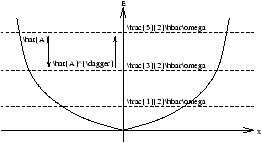
| e0= |
|
® E0= |
|
w (15.7) |
| En= |
æ ç ç è |
n+ |
|
ö ÷ ÷ ø |
w (15.8) |
|
æ ç ç è |
b + |
|
ö ÷ ÷ ø |
Y0(b )=0 |
| Þ |
|
Yn(b )=-bY0(b ) (15.9) |
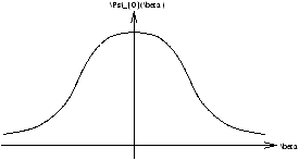
| Y0(b )=C0e |
|
(15.10) |
| C0= |
|
= |
æ ç ç è |
|
ö ÷ ÷ ø |
|
(15.11) |
| Y0(x)= |
æ ç ç è |
|
ö ÷ ÷ ø |
|
e |
|
(15.12) |
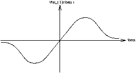
| A | Y0(b )µY1(b ) |
| Y1(b )µ |
|
æ ç ç è |
b - |
|
ö ÷ ÷ ø |
C0e |
|
| Þ Y1(b )µ |
|
(2b )e |
|
(15.13) |
| Y2(b )µ (A | )2Y0(b ) [A | applied twice] |
| Þ Y2(b )µ C0 |
æ ç ç è |
|
ö ÷ ÷ ø |
|
(4b2-2)e |
|
(15.14) |