Chapter 12 Lecture 11 - Finite Square Well

12.1 Characteristics of Well

Figure 11.1 - The Finite Square Well

This is an important problem for realistic treatments of

certain nuclear potentials
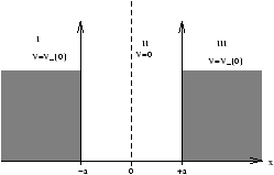
quantum well structures

In a classical sense

E>V₀ :: then the particle is free (has continous energy)
E<V₀ :: then the particle is bound (has quantised energy)

In region II where V(x)=0 we can say

Y_II(x)=Acos(ka)+Bsin(kx) (12.1)

where k=(2mE/²)^1/2 , this comes from equations III.3 and III.4.

In regions I and III where V(x)=V₀ we get

dx²

Y (x)=(V₀-E)Y (x) (12.2)

the general solutions of this are

Y_I,III=Ce^Kx+De^-Kx (12.3)

æ
ç
ç
è

2m(V₀-E)

ö
÷
÷
ø

(12.4)

If K is an imaginary quantity then E>V₀ and so free, however if K is a real quantity then E<V₀ .

12.2 Form of Energy Eigenfunctions

For E<V₀ :

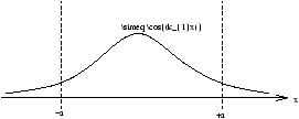
Y_I,III(x)~ e^-K|x| , this provides the expontial decay
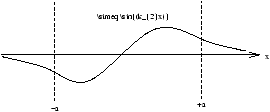
Y_II(x)~[_sin_(kx)^cos^(kx)]

Figure 11.2 - n=1 (Lowest Energy Solution) For the Finite Well. This is Said To Have Even Parity as it is Symmetric.

Note that in a classical model the regions beyond -a and +a would be void of the particle, however Schrödinger's Equation says otherwise.

Figure 11.3 - n=2 For the Finite Well. This is Said To Have Odd Parity as it is Anti-Symmetric.

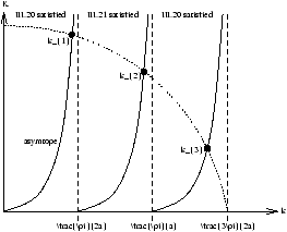
12.3 Determination of Energy Eigenvalues

For E<V₀ :

no general analytically solutions to this problem exist however it can be solved numerically or graphically. We will be looking at the graphical solution later
boundary conditions (from lecture 10)

condition i:

lim

x®¥
Y (x)® 0     (12.5)
this restricts Y_I and Y_III to
Y_I(x)=Ce^Kx Y_III(x)=De^-Kx     (12.6)

condition i and iii
states we need Y (x) and d/dxY (x) to be continous

Y_I(-a)=Y_III(-a)

d

dx
Y_I(-a)=

d

dx
Y_III(-a)     (12.7)

at x=-a: Acos(ka)-Bsin(ka)=Ce^-Ka  (a) kAsin(ka)+kBcos(ka)=KCe^-Ka  (b) at x=a: Acos(ka)+Bsin(ka)=Ce^-Ka  (c) -kAsin(ka)+kBcos(ka)=-KCe^-Ka  (d)     (12.8)
if we now rearrange (eg. (a)+(c))
2Acos(ka)=(C+D)e^-Ka  (a) 2kAsin(ka)=K(C+D)e^-Ka  (b) 2Bsin(ka)=(D-C)e^-Ka  (c) 2kAcos(ka)=-K(D-C)e^-Ka  (d)     (12.9)

As for Y_II

Y_II(x)µcos(ka) where B=0 , thus we can take (b)/(a)
ktan(ka)=K (12.10)
Y_II(x)µsin(ka) where A=0 , this we can take (d)/(c)
kcot(ka)=-K (12.11)

for the cos solutions equation III.20 must be satisfied whilst for the sin solutions equation III.21 must be satisfied.

Additionally from the definition of k and K

k²+K²=

V₀ (12.12)

12.4 Graphically Obtained Solution

Figure 11.4 - Whats Happening Graphically

As V₀ gets bigger so does the circle and therefore more solutions for the intersects k_n (eignenstates) exist. Properties of this

there is always at least one bound state
E_n(V₀)<E_n(¥ )
for large V₀ we can approximate to E₁(V₀)~ E₁(¥ )