


| - |
|
|
Y (x)+V(x)Y (x)=EY (x) |
| - |
|
|
Y (x)=EY (x) (11.1) |
| E= |
|
| Þ |
|
Y (x)=- |
æ ç ç è |
|
ö ÷ ÷ ø |
|
Y (x) |
| Y (x)=C1e |
|
+C2e |
|
=C1'sin |
|
+C2'cos |
|
(11.2) |
| - |
|
|
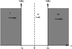
Y (x)=EY (x) |
| k= |
|
= |
æ ç ç è |
|
ö ÷ ÷ ø |
|
(11.4) |
| ka= |
|
(n=odd integers) k= |
|
(11.6) |
| ka= |
|
(n=even integers) k= |
|
(11.7) |
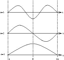
| sin |
|
n=even cos |
|
n=odd (11.8) |
| En= |
|
= |
|
(11.9) |
| Y (x)=C |
é ê ê ë |
|
ù ú ú û |
æ ç ç è |
|
x |
ö ÷ ÷ ø |
| C2 | ó õ |
|
sin2 |
æ ç ç è |
|
x |
ö ÷ ÷ ø |
dx=1 C2 | ó õ |
|
cos2 |
æ ç ç è |
|
x |
ö ÷ ÷ ø |
dx=1 (11.10) |
| Þ C= |
|
(11.11) |
| |Y (x)|2= |
|
é ê ê ë |
|
ù ú ú û |
|
æ ç ç è |
|
x |
ö ÷ ÷ ø |
(11.12) |
| En= |
|
(for n=1) |