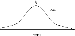
Previous Contents Next

Chapter 10   Summary 1

10.1   General Meanings


Figure Sum1.1 - The Wavefunction Y (x,t)
If the wavefunction is normalised than the probability amplitude is
|Y (x,t)|2
as the particle has to be somewhere we can say
ó
õ
¥


-¥
|Y (x,y)|2dx=1
however the particles location can be averaged
x = ó
õ
dx.x.P(x)
similarly we can write
x2 = ó
õ
dx.x2.P(x)
from this we can calculate the distribution variance (dispersion), this is similar to the standard deviation
[x2=]  s2=x2-x

The expectation value of the wavefunction is
x = ó
õ
dx.|Y (x,t)|2

10.2   Operators

When dealing with the quantum world we need a way to relate the quantum world to our world
x® X.x
this translates the quantum world to something we can grasp
XY (x,t)=xY (x,t)
A = ó
õ
dx[Af(x)]*g(x)= ó
õ
dx.f(x)*[Ag(x)]
recalling that the scaler product ( |f||g|cos(ab) ) can be used to
ó
õ
¥


-¥
dxf*(x)g(x)º f.gº <f|g>

(Af.g)=(f.Ag)

now if we consider momentum, to describe the particles motion we use
Ce
 
(px-Et)
 

Þ æ
ç
ç
è
-
x
ö
÷
÷
ø
Ce
 
(px-Et)
 
=pCe
 
(px-Et)
 
p=-
x
pY =pY
ó
õ
¥


-¥
dx.Y*(x,t) æ
ç
ç
è
-
 
.
x
ö
÷
÷
ø
Y (x,t)= ó
õ
¥


-¥
dx é
ê
ê
ë
æ
ç
ç
è
-
 
.
x
ö
÷
÷
ø
Y*(x,t) ù
ú
ú
û
Y (x,t)

10.3   Generic Hermition Functions

Afn=anfn
where A is the operator, fn is the eigenfunction and an is the eigenstate. Therefore we can say
Þ ó
õ
¥


-¥
dx.fn*(x)fm(x)=dnm
where dnm=0 if n¹ m and dnm=1 if n=m .

This is because A®A where A involves sets of eigenstates Â{ a1, a2, ... , an } and eigenfunctions { f1, f2, ... , fn} .

Note that so far we have considered all our integrals to cover all of space however they could instead be boundaries such as a well.

P(am|Y (x))=| ó
õ
¥


-¥
dx.fn*(x)Y (x)|2
this comes from the eigenfunction (the state) which provides us a measurement we would obtain with the corresponding eigenvalue
Y (x)=f3(x) Þ a3
system=state Þ measurement

what if Y (x)=f1(x)+f2(x)/2
Þ p(an|Y (x))=
1
2
| ó
õ
¥


-¥
dx.dn1+ ó
õ
¥


-¥
dx.dn2|2
p(a1)=
1
2
p(a2)=
1
2
p(an)=0  (n¹ 1,2)

now from x=ò dxY*(x)xY (x) we get
<A >= ó
õ
dxY*(x)AY (x)
when acted upon by a particular state
Y (x)=
n
å
n=1
cnfn(x)

Þ ó
õ
dx
æ
ç
ç
è
n
å
i=1
ci*fi*(x)A ö
÷
÷
ø
æ
ç
ç
è
n
å
j=1
cjfj(x) ö
÷
÷
ø
= ó
õ
dx
n
å
i=1
n
å
j=1
ci*cjfi*(x)fj*(x)aj
however as ò-¥¥dx.fn*(x)fm(x)=dnm we obtain

ó
õ
dx
æ
ç
ç
è
n
å
i=1
ci*fi*(x)A ö
÷
÷
ø
æ
ç
ç
è
n
å
j=1
cjfj(x) ö
÷
÷
ø
=
n
å
i=1
|ci|2ai=
n
å
i=1
aip(ai|Y )
p(ai|Y )=|ci|2  (the probability amplitude)

so we can conclude for the eigenstates { a1, a2, ... , an } and probability amplitudes { p(a1), p(a2), ... , p(an) }
<A >=
n
å
i=1
aip(ai)=weighted sum

Previous Contents Next