


| Ñ .E=0 Ñ .B=0 Ñ×E=-µ |
|
Ñ×H=jf+e |
|
(5.1) |
| Ñ× (Ñ×E)=-µ |
|
Ñ×H |
| Ñ (Ñ .E)-Ñ2E=-µ |
|
æ ç ç è |
e |
|
+sE |
ö ÷ ÷ ø |
| Ñ2E=µs |
|
+µe |
|
(5.3) |
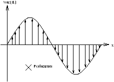
| E | (x,t)=E0e |
|
y (5.4) |
|
= |
|
+1 (5.5) |
| E | (x,t)=E0e |
|
e |
|
y (5.6) |
| Ñ×H=sE+e |
|
| |sE|>> |
½ ½ ½ ½ |
e |
|
½ ½ ½ ½ |
|
~ 1012 |
|
= |
|
| -k=w |
|
| =e |
|
| =e |
|
=cos |
|
+sin |
|
| = |
|
| k=w (1+ ) |
æ ç ç è |
|
ö ÷ ÷ ø |
|
(5.8) |
| kc= |
æ ç ç è |
|
ö ÷ ÷ ø |
|
(kc>>kvacuum) |
| E | (x,t)=E0e |
|
e |
|
y (5.9) |
| vp= |
|
= |
|
= |
|
(5.10) |
|
= |
|
<<1 |
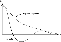
| d = |
|
= |
|
(5.11) |
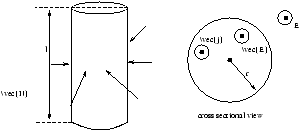
| I=s v |
|
= |
|
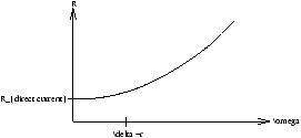
| Rdirect current= |
|
| I= | ó õj.dS |
=s | ó õE.dS |
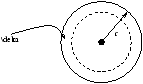
| Rhigh frequency= |
|
= |
|
= |
|
| Rhigh frequency= |
|
|
(5.12) |
|
= |
|
<<1 |
| H= |
|
(x×E) |
| H= |
|
E0e |
|
e |
|
z |
| H= |
|
E0e |
|
e |
|
z (5.13) |
| ZC= |
|
= |
|
e |
|
| e |
|
= |
|
| Zc=(1- ) |
|
=(1- ) |
|
(5.14) |
|
= |
|
|
=(1- ) |
|
=(1- ) a |
|
= |
|
|
= |
|
|
=- |
|
~ -1 |
| R= |
½ ½ ½ ½ |
|
½ ½ ½ ½ |
~ 1-4a |
| R=1-2 |
|
(5.15) |