


Chapter 2 Interaction of Radiation With Atoms
2.1 Spectroscopy (see the handout)
2.2 Einstein A and B Coefficients
Spectroscopy assumes two processes
-
spontaneous emission
- absorbsion
imagine a two level atom
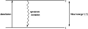
Figure 3.1 - A Two Level Atom
The probability per unit time that a photon will be spontaneously emitted is A21 s-1 . We need Quantum ElectroDynamics to calculate A21 . A21~ 108s-1 for a strong transition however the probability per unit time that a photon will be absorbed it proportional to r (w )=B12r (w ) . So it depends on how strong the radiation field is
| r (w )= |
|
per unit frequency interval |
N=N1+N2 (2.1)
where N1 is the number in state one and N2 is the number in state 2.
|
|
|
=- |
|
=A21N2-B12r (w ) N1 (2.2) |
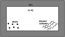
Figure 3.2 - A Box Containing Two Level Atom's
We now consider the situation in figure 3.2 so at thermal equilibrium
which results in
equation 3.3 implies that if r (w ) is big then N2 is much greater than N1 and all the population is in the excited state, however this does not agree with thermodynamics. In thermal equilibrium
so a big r (w ) occurs at high T , now Boltzmann says
at a high value of T , N2~ N1 , so half the population is in the excited state. Einstein proposed a third process
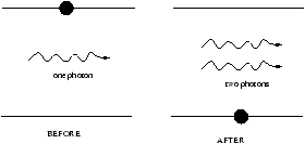
Figure 3.3 - Stimulated Emission
The probability per unit time that the stimulated emission will occur is proportional to r (w )=B21r (w ) . For an ensemble
|
|
|
=A21N2-B12r (w )N1+B21r (w )N2 (2.6) |
| |
|
= |
|
= |
| B12 |
|
æ
ç
ç
ç
ç
ç
ç
è |
| A21p2c3 |
|
| w123 |
æ
ç
ç
ç
è |
e |
|
-1 |
ö
÷
÷
÷
ø |
+B21 |
|
|
ö
÷
÷
÷
÷
÷
÷
ø |
|
|
|
B12=B21 and |
|
A21=B21 (2.8) |
2.2.1 Saturation
from equations 3.7 and 3.1 we can obtain
So as r®¥ we get N2/N®1/2 .
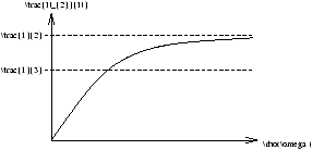
Figure 3.4 - ???
the saturation intensity is defined to occur when Brsaturation=A . If we substitute this into equation 3.9 we get
note that for an optical transistion w~ 5® 10 eV , at room temperature kT~1/40eV so we can conclude that nearly all the population is in the ground state at room temperature.
2.2.2 Natural Lifetime
In the absence of external driving radiation (where r (w )=0 ), equation 3.2 gives
the natural lifetime t2=1/A21 for a two level atom. IF the atom is not a two level atom then
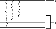
Figure 3.5 - A Non Two Level Atom System
ti=1/åjAij which is typically t~ 10-8s .
2.3 Spectral Line Broadening
2.3.1 Natural Broadening
Due to spontaneous emission, ie. QED (Quantum Electodynamics Effect). The classical picture states the atom is an oscillating dipole with an exponential decay.
where g =1/t=A21 for a two level atom.
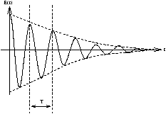
Figure 3.6 - A Classical Explanation For Natural Broadening (ratio of
T:
t is greatly exaggerated)
E(w ) comes from the Fourier Transform of E(t)
I(w )~ |E(w )|2
equation 3.10 is known as the Lorentzian.
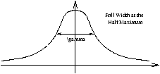
Figure 3.7 - Gaussian to
g Translation
2.3.2 Doppler Broadening
In atomic spectroscopy the samples used are in the form of gases where the atoms move randomly.
where r is the unit vector from the observer to the atom. The velocity distribution is Maxwellian (ie. Gaussian)
a depends on the atomic weight ( A ).
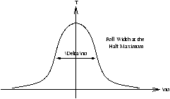
Figure 3.8 - ???
|
|
|
=7× 10⁻⁷ |
æ
ç
ç
è |
|
ö
÷
÷
ø |
|
(2.11) |
2.3.3 Pressure Broadening (Collision Broadening)
In the classical picture, similar to the Natual Broadening case however this time with collisions, the light consists of blocks of radiation of length Tc where the length is the time between collisions (this is random motion). For one block
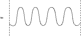
Figure 3.9 - Pressure Broadening
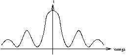
Figure 3.10 - The Classical Picture of a Collisioned
I(
w )
which is Lorentzian again where gc is the collision width.
A rule of thumb gives us that
2.4 Selection Rules
If
the transistion from one to two is forbidden. We saw that Z12=0 for Y1º 1s state of hydrogen and Y2º 2s state of hydrogen. However for Z¹ 0 then Y1º 1s state of hydrogen and Y2º 2p state of hydrogen ( Ml=0 ).
The physical interpretation for 1s-2p ( Ml=0 ) the superposition wavefunction (from section 3.4, equation 4) leads to a lopsided oscillating charge cloud. This resembles a classical oscillating dipole. For 1s-2s superposition wavefunction forms a spherically symmetrical charge cloud. This does not look like a dipole
-
Rule One:
- the electic dipole transitions can only occur between states of opposite parity. This is also known as Laporle's Rule.
The selection rule results when Z12=0 . If we examine Z12 in detail we find other ways Z12 can vanish. We recall that
Ynlm=Rne(r)Ylm(q ,f )
The parity of Ylm is (-1)l . This leads to
Ylm(p -q ,q+p )=(-1)lYlm(q ,f )
under Laporle's rule
-
s-s:
- is forbidden
- s-p:
- is allowed
- s-d:
- is forbidden
- s-f:
- is allowed
but s-f does not occur, so we look again at Z12
| Z12= |
ó
õ Rnl(r)Ylm*(q ,f )zRnl(r)Ylm(q ,f )dV |
2.4.1 theta integral
The q dependence of Ylm is complicated however we will just quote the result. The q integral is zero unless D l=l'-l=± 1 .
-
Rule Two:
- D l=± 1
the physical interpretation is that a photon carries one unit of angular momentum however overall angular momentum (atoms and radiation) must be conserved so l can only change by 1 .
2.4.2 phi integral
We assume that the light is linearly polarised with E polarised along the z-axis. For this case it can be shown that the f integral is:
Therefore D m=0 is allowed for this polatisation, however we note that this agrees with our example with Y2º 2p when Ml=0 .
Only one other circumstance gives an allowed transistion, circular polarised light with E in the x-y plane. This gives use D M=± 1 (this depends on the handedness of circular polarisation).
-
Rule Three:
- D Ml=0,± 1 is known as the Zeeman's effect
2.4.3 r integral
The r integral never vanishes and it depends on n
-
Rule Four:
- D n=anything
2.5 Metastable States
If there is no lower state to which an excited atom can make an allowed transition then the state should in principle be stable. The breakdown of the electric dipole approximation leads to weak radiation. The state is said to be metastable. For example the 2s state of hydrogen with a natural lifetime t~1/7s .