

|
=R |
æ ç ç è |
|
- |
|
ö ÷ ÷ ø |
(1.1) |
| Þ |
|
= |
|
(1.2) |
| r=n2a0, a0= |
|
(1.4) |
| n = |
|
(1.5) |
| E=T+V= |
|
mev2- |
|
| E=- |
|
hc, R |
|
= |
|
|
|
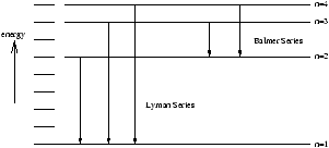
| D E=E |
|
-E |
|
=hcR |
|
æ ç ç è |
|
- |
|
ö ÷ ÷ ø |
| D E=hn = |
|
| me® m= |
|
|
=R |
æ ç ç è |
|
- |
|
ö ÷ ÷ ø |
= |
|
R |
|
é ê ê ë |
- |
|
Ñ2+V(r) |
ù ú ú û |
Y (r)=EY (r) (1.6) |
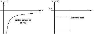
| V(r)=V(r)=- |
|
(1.7) |
| Ñ2= |
|
é ê ê ë |
|
æ ç ç è |
r2 |
|
ö ÷ ÷ ø |
+(q ,f ) |
ù ú ú û |
(1.8) |
| (q ,f )= |
|
|
+ |
|
|
æ ç ç è |
sinq |
|
ö ÷ ÷ ø |
(1.9) |
|
|
æ ç ç è |
r2 |
|
R |
ö ÷ ÷ ø |
- |
|
r2+ |
|
r2=- |
|
(q ,f )Y (1.11) |
|
|
æ ç ç è |
r2 |
|
R |
ö ÷ ÷ ø |
+ |
|
- |
|
=c1 (1.12) |
| - |
|
(q ,f )Y=c1 (1.13) |
| - |
|
|
=c2 (1.14) |
|
|
æ ç ç è |
sinq |
|
ö ÷ ÷ ø |
+c1sin2q=c2 (1.15) |
| F = |
|
e |
|
; me=0,± integer (1.16) |
|
é ê ê ë |
(1-e2) |
|
ù ú ú û |
+c1F=0 (1.17) |
| F(e )= |
|
anek (1.18) |
| ak+2= |
é ê ê ë |
|
ù ú ú û |
ak (1.19) |
| - |
|
|
(1.20) |
|
é ê ê ë |
- |
|
|
+Veffective |
ù ú ú û |
P(r)=EP(r) (1.21) |
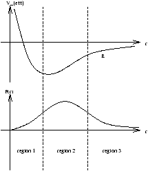
| Veffective=- |
|
+ |
|
(1.22) |
| Veffective=V+ |
|
| r= |
|
| l = |
|
(1.23) |
| a2=- |
|
(1.24) |
|
é ê ê ë |
|
+ |
|
- |
|
- |
|
ù ú ú û |
P(r )=0 (1.25) |
|
é ê ê ë |
|
- |
|
ù ú ú û |
P=0 (1.26) |
|
é ê ê ë |
|
- |
|
ù ú ú û |
(1.27) |
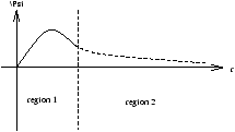
| g(r )= |
|
ckrk |
| P~ | e |
|
rl+1g(r ) (1.28) |
| E=- |
|
| lz=- |
|
| l2=-2 |
é ê ê ë |
|
|
æ ç ç è |
sinq |
|
ö ÷ ÷ ø |
+ |
|
|
ù ú ú û |
| l | 2Y |
|
=l(l+1)2Y |
|
, l=0,1,2,... |
| l | zY |
|
=Ml Y |
|
, Ml=l,l-1,l-2,... ,-l |