


Chapter 2 The Beginnings of Wave Mechanics
The photoelectric effect, Bohr model and Compton scattering showed that when EM
waves interact with matter they behave like particles. In free space they behave like waves. Therefore EM radiation demonstrates a Wave-Particle Duality.
2.1 de Broglie
In a significant early example of the use of symmetry in physics, de Broglie (1924) proposed that particles of matter should also have wave properties; ie. wave-particle duality extends to matter. Specifically he proposed that equations 1.12 and ??1.35?? which apply to photons also apply to matter. ie.
This is the de Broglie relationship.
He also proposed that if the particle has total energy E , then
E=hf
(2.2)
gives the frequency of the wave.
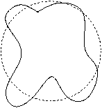
Figure 2.1
An electron in a Bohr orbit with fixed p , and hence l , will form a standing wave; ie. there must be n whole number of wavelengths fitting into the circumference
2p r=nl where: n=1,2,3,...
substituting from equation 2.1
|
rp=mevr=n |
æ
ç
ç
è |
|
ö
÷
÷
ø |
=n
(2.3) |
Angular momentum quantisation explained integral numbers of l must fit into the circumference. It also goes some way to explaining the stationary states of Bohr's 1st postulate.
An electron can only change from one orbit to another if there are integral changes in angular momentum, therefore energy connot change continously.
In 1926 Daineon and Germer showed experimentally that electrons were diffracted by a crystal. The regular atomic spacing acts like a diffraction grating. They were scattering electrons which had been accelerated by a potential difference of V0 volts.
| KE= |
|
=eV0 the loss in potential energy |
Classwork III - shows that this non-relativistic treatment is justified.
2.2 Schrödinger's Wave Equation
Before we introduce Schrödinger's Wave Equation we must change f and l to the variables used in optics.
w (angular frequency)=2p f
(2.6)
In an EM wave, equation 1.10 states c=fl
Equation 2.7 does not hold for matter waves. de Broglie's relationship (equation 2.1) becomes:
Planck's relationship (equation 2.1) becomes
From Waves and Optics we know the wave equation for EM, sound waves and waves on a string,
with solutions which are travelling waves in the positive x direction.
|
y=De |
|
=D(cos(kx-w t)+sin(kx-w t))
(2.11) |
-
a travelling particle wave can be represented by a wave function which can be represented as
- the wave function is well behaved mathematically (differentiable)
- a matter wabe equation whould be linear (no terms in Y2 or (dY/dx)2 etc) so that the principle of linear superposition holds, as it does for equation 2.10 (this is important in Wave and Optics)
- assumed de Broglie equations 2.1 and 2.2 applies
- assumed, non-relativistic expressions
2.2.1 Schrödinger's Equation (aka Handout III)
Schrödinger's Equation should be regarded as a postulate. Like Newton's Laws, Maxwell's Equations, Special Relativity, it cannot be derived from more basic principles. Its justification comes from giving solutions which agree with experiments. As discussed, Schrödinger based his equation on Hamilton's principle of least action. We will see how a wave equation can be derived which has solutions which are travelling waves.
| Y (x,t)=Ae |
|
(equation 2.12) |
p= k (equation 2.8)
Schrödinger realised there is a problem if equation 2.2, E=hf holds, using equation 2.9
If equation 2.12 is to be a solution of a wave equation like equation 2.10 (see Waves and Optics) it will have to be differentiated twice with respect to x and twice with respect to time. ie. factors of k2 and w2 will appear which will not be easy to relate, given that equation 2.13 contains w and k2 .
Schrödinger therefore guessed that the wave equation would include the first derivative with respect to time. To be correct relativistically one woul need to treat x and t in the same way, but then Schrödinger was assuming a non-relativistic approach. Rearranging equation 2.13
Differentiate Y in equation 2.12 twice with respect to x
| |
|
Y (x,t)=A k |
|
e |
|
=A( k)2e |
|
=-k2Y (x,t) |
| |
|
Y (x,t)=- |
|
(E-U(x))Y (x,t) |
|
- |
|
× |
|
Y (x,t)+U(x)Y (x,t)=EY (x,t)
(2.15) |
| |
|
Y (x,t)= |
|
Ae |
|
=A(- w)e |
|
=-wY (x,t) |
|
|
æ
ç
ç
è |
- |
|
× |
|
+U(x) |
ö
÷
÷
ø |
Y (x,t)=EY (x,t)= |
|
Y (x,t)
(2.17) |
|
|
æ
ç
ç
è |
- |
|
× |
|
+U(x) |
ö
÷
÷
ø |
Y (x)=EY (x)
(2.20) |
Energy Conservation
Energy conservation holds in its non-relativistic term. He realised the problem with equation ??1.34?? that
ie. if we fix p from p=h/l you get both positive and negative energy states. The problem was solved by Dirac by filling all negative
energy states with electrons and relying on the Pauli Exclusion Principle. Schrödinger applied a least-action principle. More significantly Schrödinger argued that for EM waves Fermat's principle applies (least-time) and describes how light rays behave. The equivalent for particles is Hamilton's principle
of least action.
Schrödinger was searching for the matter equivalent of the Huygens-Fiesael principle that light waves on a small scale add up to wave fronts and rays on the large scale, where they obey Fermat's principle.
2.3 The interpretation of the Wave Function
particles are waves in/of what?
Einstein's view of EM radiation was that for fixed f the intensity of light at a point which classically depends on the square of the amplitude of the EM wave is proportional to the number of photons.
By analogy Max Born (1926) suggested the square of the Schrödinger wave function in a small volume dV is proportional to the probability of finding the particle in dV .
In one dimension the probability of finding a particle between x and x+dx is proportional to the square of the amplitude (which can be complex). eg.
µ |Y |2dx=Y '(x)Y(x)dx
(2.21)
For particles like electons which are conserved (ie. total number constant) and so has to be somewher we fix arbitrary constants such as A in equation 2.19 by normalisation condition
|
|
ó
õ |
|
Y* (x)Y (x)dx=1
(2.22) |
2.4 Recipe for Solving Schrödinger's Equation
-
sketch U(x) (the potential) and divide into approiate regions
- set up Schrödinger's equation in each region
- guess Y (x) in each region with two arbitrary constants as equation 2.20 has second derivitives
- work out d2Y/dx2 substitute in equation 2.20 to find an approiate k
- impose boundary conditions at the limits of each region
-
the wave function should be contineous at the boundary
- dY/dx should be contineous at the boundary.
These conditions result from the Schrödinger assumption II ( Y must be well behaved mathematically). If condition 2 doesn't hold d2Y/dx2 can become infinite therefore infinite energy
- as x® ¥ , Y must be finite to keep equation 2.22 possible
2.5 The Infinite Square Potential Well
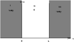
Figure 2.2
This is no loger just an academic excerise. Nowadays its possible to change the conduction band edge of a semiconductor from one atomic layer to the next be Moleculat Beam Epitaxy (MBE).
A Quantum Well a few nanometers wide can be formed between high band gap barriers.
Solve equation 2.20 for a particle of mass m confined in this well (eg. an electron).
-
sketch (figure 2.2)
- label regions
In region II, 0<x<L , U(x)=0
- looks like SHM therefore we will make an educated guess that
Y =Asin(kx+f )
(2.24)
- differentiate twice
|
E= |
|
= |
|
(by de Broylie (equation 2.8))
(2.25) |
- the boundary condition if U(0)®¥ and U(L)®¥ the electron cannnot exist outside the well. On the probability interpretation of Y (x) expect
Y (0)=0; Y (L)=0
-
x=0; Y (0)=0
from equation 2.24:
0=Asinf f=0
- x=L; Y (L)=0
from equation 2.24:
kL=np; n=1,2,3,...
substitute into equation 2.25
Note that:
-
on the Schrödinger picture it is the boundary condition which produce quantisation
- there is a series of energy levels. The spacing increases like n2 , compared to the Bohr atom where Enµ1/n2 (equation 1.25)
- the electron can't have zero energy, the lowest energy level is 2p/2mL2
this lowest energy is know as the
-
zero point energy
- confinment energy
The wave functions correspond to different values of n and En are found by substituting equation 2.26 into equation 2.24 with f =0
|
Y (x)=Un(x)=Asin |
æ
ç
ç
è |
|
x |
ö
÷
÷
ø |
n=1,2,3,...
(2.28) |
To emphasise that, in this case, the wave functions correspond to definate values of En and for reasons which will be clearer when we get to Formal Quantum Mechanics (section 3) these functions are also called energy eigenfunctions (Un(x)) and the corresponding En are known as energy eigenvalues.
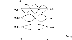
Figure 2.3
The first three energy levels E1 , E2 , E3 are plotted in figure 2.3 and the corresponding Un are sketched at each En .
Just as in figure 2.1 when an electron is confined in a small region of space it forms standing waves. Again, there is a quantum number associated with the standing wave.
Note that the Un (x) are orthogonal.
|
|
ó
õ |
|
Ym*(x)Y (x)dx=0 if m n
(2.29) |

Figure 2.4
Figure 2.4 shows the probability distribution, note one electron in the n=2 level has zero probability of being at the well's centre and equal probability of being on the left and right hand side.
For high speed amplifiers (eg. satelite dish) have electrons moving at high speed along the well (perpendicular to figure 2.4).
If you grow a single monolayer plane of scattering atoms at the centre of say an 11-monolayer wide well the speed of the electrons in the n=2 level are not affected but electrons in the n=1 and n=3 levels slow down.
2.6 Finite Square Well
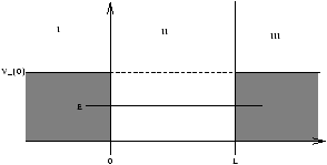
Figure 2.5
-
sketch well with finite barrier V0 as in figure 2.5
- in regions I and III Schrödinger's equation 2.20 becomes
| - |
|
× |
|
+V0Y=EY (from equation 2.23) |
However Quantum Mechanically things are different as recipe stages 3,4 and 5 will show.
- in regions I and III (guess)
Y =CeKx+De-Kx
(2.31)
-
| |
|
=CK2eKx+DK2e-Kx=K2 |
( |
CeKx+De-Kx |
) |
=K2Y |
- consider boundary conditions to regions I and III as x®±¥ .
-
in region III:
- C=0 otherwise Y3®¥ as x® +¥
- in region I:
- D=0 otherwise Y1®¥ as x® -¥
- in region III:
-
Y3=De-Kx, x³ L
(2.33)
- in region I:
-
Y1=CeKx, x£ 0
(2.34)
- in region II:
- we expect Y2=Asin(kx+f ) with K2=2mE/2 (from equation 2.24).
equivalently we can use
At x=0 , continuity of Y and dY/dx give two equations for A, B and C.
At x=L , continuity of Y and dY/dx give two equations for A, B and D.
Therefore four equations with four unknowns can be solved to give solutions.
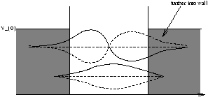
Figure 2.6
Note as V0®¥ , Y® Un of figure 2.3. Also as E® V0 , Y penetrates further into the barrier as in figure 2.6.
2.6.1 Quantum Tunneling
The exponential decay of electon waves in a classically forbidden region is equivalent to total internal reflection from Waves and Optics.
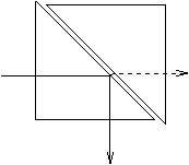
Figure 2.7
A rapidly decaying EM wave (the evanescent wave) penetrates a short distance into the lower refractive index medium. A second prism (as shown in figure 2.7) willpick up some light if close enough. If a second region like II is brought up into region I or III where the electron wave is still finite an oscillating solution resumes outside the barrier known as quantum mechanical tunneling. This process is also responsible for alpha particle decay.
2.7 Uncertainity in Quantum Mechanics
To find where an electron is we will need to do an experiment eg. shine light on it.
Optics says you can't determine the position of an object or its size with light of wavelength l to better than the size of the diffraction limited spot. Therefore the uncertainity in the electrons position:
D x l
(2.36)
But light of wavelength l has momentum
and when it shines on the electron it will scatter as in the Compton effect changing the electron's momentum from zero (assumed) to P'E .
| P |
|
=P |
' |
|
+P'E (from equation 1.36) |
D xD Px h
(2.38)
This is Hesenberg's Uncertainity Principle1 which also applies to energy and time2
D ED t h
(2.39)
Note that if we reduce l to fix the objects position better we give the electron a bigger kick and so D Px becomes larger.
2.8 Wave Packets
Assumption III in Schrödinger's Equation was that the equation had to be linear so as in Wave and Optics two solutions of Schrödinger's equation when added also form a solution. Superposition applies.
In Wave Optics superposition of waves of different wavelength's leads to the formation of wave packets or pulse. The individual waves have phase velocity v=w/k (as in equation 2.7).
The envelope of the ave packet with the group velocity is
In Wave and Optics the range of frequencies Dw which give a pulse of width D t are related by the bandwidth theorem.
D tD w~ 2p
(2.41)
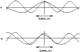
Figure 2.8
Figure 2.8 is a pulse centred at x=0 can be built up starting with a wave of wavelength l0 . Superimposing a wave of wavelength 2l0 will cancel out the maxima nearest x=0 but reinforce the next. Another wave of wavelength 4l0/5 will reduce the second maxima.
The smaller the pulse wifth D x the more wavelengths needed therefore the bigger wavelength spread Dl .
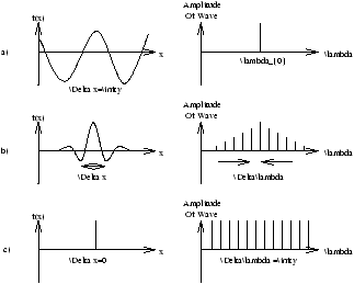
The Situation is Summarised
Figure 2.9
Multiply both sides of equation 2.41 by and use equation 2.9 ( E= t ).
D tDw=D tD E= 2p =h
We get the uncertainity principle (equation 2.39) this also helps explain wave particle duality. Electrons and EM waves can be represented as wave packets when behaving as particles
Consider a free electron (ie. zero potential energy) moving with non-relativistic energy:
It should be pictured as a wave packet moving with group velocity
remember equation 2.8, p= k , therefore the electron wave packet moves
which is the non-relativistic particle speed.
- 1
- Different textbooks divide the right hand side by 2 or 2p
- 2
- Different textbooks divide the right hand side by 2 or 2p