


Chapter 1 Light
1.1 Waves or Particles?
In the 17th century Newton thought light was a stream of particles or corpusles.
In 1802 Young showed by using two slit interference experiments that light has a wave function (nature).
A particle moves at constant speed relative to its sources. eg. a bullet fired in a train will also aquire the speed of its source.
A wave moves at constant speed relative to the medium in which it propagates (eg. sound).
If light was a particle then the light from a binary star moving towards the observer would move faster then when that component star moved away this distortion to the orbits of binary stars was not observed therefore light is not a particle.
In 1865 Maxwell unified electricty and magnetism into electromagnetism (EM) wand in doing so showed that light was an EM wave.
The medium in which light propagates in must be rigid as the waves travel very fast but it does't show the earths motion. When physicists don't understand something it is given a name, the Ether.
If light is a wave motion it should have constant speed relative to the ether and it should be possible to detect this motion with the classical Doppler Effect. Around 1887 Michelson and Morley looked for a frequency shift due to the earths motion through the ether - the speed was zero.
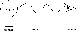
Figure 1.1
Instead of the speed of light begin relative to the source (or medium) it is relative to the observer.
In 1905 Einstein wrote his postulates. His 2nd postulate shows that light from a binary star in not relative to the source. The Michelson-Morley experiment says not relative to the medium. So if the speed of light is to have a meaning it must be constant relative to something. Einstein postulatedthat the speed of light was constant relative to the observer.
Points worth mentioning
-
this is the first time in physics that the observer matters. In QM we find the observer matters a lot
- the breakdown of classical physics mainly involves the interaction of radiation with matter
- we will find eventually that light behaves both as a wave and particle
1.2 Blackbody Radiation
It is not easy to measure how much radiation a body emits. External light could be relected. Emitted light can be reabsorbed by the body itself.
19th century physicists devised an ideal system for studying radiation emission experimentally and theoretically.
Define: An ideal blackbody is a system which absorbs al radiation incident on it (ie. no reflection)
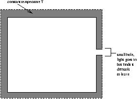
Figure 1.2
They realised that a small opending in an otherwise closed cavity which was constant temperature T would act as an ideal black body, as anu radiation which enters is unlikely to emerge.
Note that it is the small hole which is the blackbody.
The radiant energy absorbed by the opening should lead to a rise in T , but we said the cavity is in equilibrium at constant T . To stay in equilibrium the opening must emit an exactly equal and opposite amount of radiation to that which it absorbs. ie. An ideal blackbody absorber is an ideal blackbody emitter.
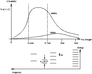
Figure 1.3
Experimental results in figure 1.3
-
the spectrum was independent of the material in the walls of the cavity, but does depend on the value of T
- the total intensity of the radiation increases very strongly (to the 4th power) with T being related by the Stefan-Boltzmann law
I=s T4
(1.1)
where:
-
s
- is the universal constant called the Stepfan-Boltzmann constant
s = 5.67× 10⁻⁸ Wm-2K4
(1.2)
- T
- is the absolute temperature
- as T rises the intensity peak shifts to shorter wavelengths according to Wien's displacement law
lmaxT=constant
(1.3)
where:
-
constant
- is 2.9× 10⁻³ mK
The aim of the theorists was to reproduce the spectral emittance I(l) in figure 1.3 where
-
I(l)dl
- is the radiation intensity for wavelengths between l and l +dl
- I(l)
- is related to the total intensity in equation 1.1 by the following
In 1896 Wien suggested a formula which fitted the shape
wheres the constants A and B are fitted to the data
In 1900 Lord Rayleigh (of optics fame), pointed out that Wien's I(l) was independent of T at long l where as experiments showed I(l) rises as T rises.
To calculate I(l) classically (and similarly with Planck's approach) use the following steps:
-
assume cavity is filled with EM standing waves. If the walls are electical conducting there will be nodes of the electric field at the wall
- calculate the number of standing waves with wavelength between l and l + dl which fit into a cubic cavity of side L . Standing waves are often called normal modes of oscillation of the EM field (cf. coupled oscillations in Mechanics and Relativity). This operation will give you the number of standing waves per unit volume of the cavity
where g(l) is the density of states per unit cavity volume
- equipartition of energy (Structure of Matter, section 5.5) gives the correct answer for the specific heat capacity of all solids at high T . The EM waves are in equilibrium with the walls at temperature T , therefore we assume each mode of standing wave is a degree of freedom and so has a 1/2kBT of energy. There is an electric and magnetic field therefore multiply equation 1.6 by 2. Hence the energy density U(l) is the energy per unit volume of cavity of radiation with l between l and l +dl
|
U(l)= |
æ
ç
ç
è |
|
|
kBT |
ö
÷
÷
ø |
× 2
(1.7) |
- to compare with experiment we need the flux emitted by the small opening cf. with flux of ideal gas molecules of speed n emerging through a hole in the vessel is proportional in number to a cylinder of length n (or see handout 1). Hence we expect to see flux emerging of I(l) related to density inside of U(l) by
Combining equations 1.7 and 1.8, equipartition predicts
Better than Wien at long l , however the ultraviolet catastrophe occurs at short l .
1.3 Background on Planck Distribution and Derivation
THIS ENTIRE SECTION IS NOT EXAMINABLE
Derivation of equation 1.8 (from J.J. Brehm and W.J. Mullen "Introduction to Structure of Matter", Wiley).
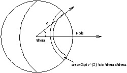
Figure 1.3-5.1
Averaging over rays with velocity components to the right
The energy flux rate I(l) and the energy density u(l) are related for cavity radiation by a proportionality factor c/4 , as in equation 1.8. We can deduce this result as the product of two contributions with the aid of figure 1.3-5.1. Tje relation calls for a factor of 1/2 because, for all the electromagnetic radiation in the cavity, only half of the standing-wae energy corresponds to rays with velocuty components to the right where the hole is located in the figure. (recall that a standing wave is an equal-parts admixture of traveling waves having opposite directions of propagation). These rays carry energy through the hole with an average velocity to the right given by the z component of the velocity of light, cz=c cosq , averaged over the right hemisphere. If we let the sphere in the figure have arbitrary radius r and average over the hemispherical area we obtain
in which we have used the substitution x=cosq . The desired relation is then found by assembling factors:
| I(l)= |
|
<cz>u= |
|
u (equation 1.8) |
The corresponding frequency distributions are related in similar fashion, in agreement with equation 1.8. We should note that the derivation does not require the cavity to have a spherical shape.
1.3.1 The Density of States for EM Waves in a Cavity
How many standing waves can be fitted into a cavity? If the cavity walls are conducting there will be nodes at the walls so the problem is like counting the number of l which can be fitted on a vibrating string. Assume the cavity is a cube of side L (the result applies to any shape). An integral number of half-wavelengths can be fitted into the cavity
where n=1,2,3,...
This holds along x , y and z axes
| k=(kx2+ky2+kz2) |
|
=(nx2+ny2+nz2) |
|
The possible k-values can be represented as equally spaced points in the 3D space in figure 1.3-5.2 (k-space). The number of k-values between k and k+dk (g(k)dk) is the number of such points in a shell of thickness dk .
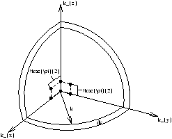
Figure 1.3-5.2
| g(k)dk= |
|
× 4p k2dk× |
æ
ç
ç
è |
|
ö
÷
÷
ø |
|
g(l)dl = g(k)dk
Each EM wave has two polarization states
1.3.2 Derivation of Planck's formula for Blackbody Radiation (1900)
Planck realised that the problem was the density of states in equation 1.6. g(l ) ® ¥ as l ® 0 . (ie. there are an infinite number of ways to fit an infinitely small l into the cavity). It was alright for long l to have 1/2kBT per mode (equation 1.9 works at high l ). How to stop the short l modes being excited?
He noted that the frequency f of the modes was given by
c=fl
(1.10)
therefore f is high for the problematic short l . In what Planck described as an act of desperation he proposed that the mode energy was given by
E=nhf where n=0,1,2,3,...
(1.11)
where h is a very small constant, now known as Planck's constant. He intended h to be a mathematical dodge whcih would give the correct result as h ® 0 .
Note the advantages of Planck's proposal:
-
Long l , low f
- the energy levels of equation 1.11 are close together so their effect is not notied. In particular the level spacing is much less than kBT and the cavity modes will be easily excited by the oscillators in the cavity walls
- Short l , high f
- energy level spacing is much greater than kBT (problem sheet I, Q3.1) oscillations in cavity walls, which have energy 1/2kBT per mode, cannot excite the standing waves.
It wasn't until later, in 1905, that Einstein pointed out that equation 1.11 meant energy was being shared between the oscillators in the walls and the EM waves in packets or quanta of size
E=hf
(1.12)
Planck used an entropy argument to get I(l ) from equation 1.11. We will use the methods of the Structure of Matter course (SoM). The number of EM modes with energy between E and E+dE is
dN=f(E)g(E)dE
We now know photons of light are bosons therefore f(E) is the Bose-Einstein distribution (often called the Planck distribution).
Note that the denominator sign is positive for the Fermi-Dirac distribution.
Substitute from equations 1.10 and 1.12
If E and E+dE corresponds to l +dl and l
dN=f(E)g(E)dE=f(l )g(l )dl
energy density
U(l )=EdN=EfBE(l )g(l )dl
substitute g(l ) from equation 1.6, E from equation 1.12, fBE(l ) from equation 1.13
using equation 1.8
This is Planck's formula for the spectral emittance. It fits all data perfectly. It agrees with Wien at short l (Problem Sheet I, Q3) and with Rayleigh-Jeans at long l (Problem Sheet 1, Q4). It was some years before Planck accepted that he had shown energy is quantised.
1.4 Photoelectric Effect
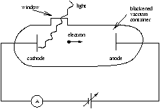
Figure 1.4
Lenard (1902) used apparatus as above to show thay monochromatic lightfalling on a cathode produces a current - photoelectric effect.
If V is the potential of the anode relative to the cathode (both same metal) he observed as in figure 1.5a:
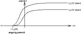
Figure 1.5a
-
whilst V is positive the current saturates at Imax when all electrons collected
- Imax is proportional to the light intensity
- whilse V is negative the electrons are repelled by the anode. When V=-V0 where V0 is the stopping potential current is zero for all intensities. At this critical point only the most energetic electrons reach the anode
|
Max KE = |
|
mvmax2=eV0
(1.16) |
Classically we expect Imax proportional light intensity as number of electrons emitted proportional light intensity.
Classically we did not expect:
-
there is no threshold in light intensity Imax µ intensity to the lowest intensities
- no observable delay in the current signal when the light was turned on, even at the lowest intensity
- there is a threshold in light frequency below f0 (figure 1.5b) there is no current
- V depends on the cathode material and on f but not on the light intensity
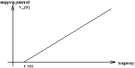
Figure 1.5b
Einstein proposed (1905) that Planck's idea to be extended to all EM radiation so that the radiation consists of discrete energy quanta (now called photons) of the size
E=hf
(1.17)
where f is the frequency of the radiation.
Light intensity at fixed f proportional to number of photons. Imax µ light intensity (as in classical description).
Einsteins approach explains:
-
no intensity threshold as one photon will eject one electron
- no delay, a single photon will eject an electron instantly
- f0 threshold - minimun energy required to extract one electron from a metal is known as the work function ( f ) usually measured in eV (electronvolts). 1eV = the energy an electron gains crossing a potential difference of one volt.
for frequencies f below f = hf the photon cannot eject an electron
(1.18)
- the maximun kinetic energy related to the photon energy
If we subsitute equations 1.18 into 1.19 to get Einsteins Photoelectric Equation
|
|
|
mvmax2=eV0=hf-f =h(f-f0)
(1.20) |
1.5 Heat Capacity of Solids
Recall from Structure of Matter thay a good model for solids is binding by Simple Harmonic Motion forces as atoms close to equilibrium. Equipartition says if 1/2kBT per quadratic degree of freedom. Specific heat of solid at constant volume CV=3R .
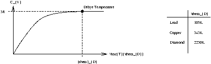
Figure 1.6 (cf Figure 16-15 p517 Young+Freedman (9th Ed))
Works for all solids at high enough temperatures
T>qD
Einstein tried to explain behaviour for T<qD by assuming atoms in solids vibrate with quantised energy spectrum with level spacing by using equation 1.12 E=hf .
Atomic vibrations will not be excited if level spacing hf» kBT ie. as T ® 0 cf. with blackbody situation cavity vibrations not excited at level spacing hf» kBT because at low l , f is large.
Debye pointed out that these vibrations are transmitted as waves (phonons) at the speed of sound.
1.6 Bohr Model of Atomic Spectre
A gas flame emits a continuous spectrum like a blackbody, of T in range 400-1000K. If T is high so that the gases ionised or there are traces of metals in the flame, line spectra are observed 1860-90, atomic spectroscopy became an exact science.
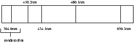
Figure 1.7 - Bamler Series Atomic Hydrogen (cf Figure 40.7, p.1237 Young+Freedman (9th Ed))
The hydrogen spectrum (figure 1.7) has four lines in the visible which Balmer (1884) fitted with a single formula Rydberg (1890) showed that a similar formula fits spectrum of the alkali metals. He suggested the formula be written for hydrogen.
where
-
m
- =3,4,5,®
- RH
- =Rydberg constant
= 1.097× 10⁻⁷ m-1
(1.22)
RH could be very well determined by measuring the wavelegth of spectrum (± 0.01%).
Bohr (1913) was aware that Thomson had shown electons were light and fundemental constituents of atoms (p.877-9 Young and Freedman (9th Ed)) and that Rutherford had shown that there was a heavy, small positively charged nucleus at the centre of the atom (p.1241-4 Young and Freedman (9th Ed)).
If you picture an atom as electons in orbit around the nucleus there are two problems resulting from the electons accelerating in orbit and hence its radiation of EM waves:
-
the electrons should spiral into the nucleus in 10-8 seconds
- electrons should radiate continously - not a line spectrum
Therefore Bohr postulated:
-
electons move only in certain circular orbits called stationary states. This motion can be described classically
- radiation only occurs when an electron jumps from an allowed orbit (total energy Em to a lower energy orbit ( En ). The radiated frequency is given by:
hf=Em-En
(1.23)
- the angular momentum of electron rest mass me is restricted to integer multiples of h/2p=
mevr=n
(1.24)
where n=1,2,3, ...
1.7 Characteristic X-Ray Spectra
X-Rays are just electromagnetic waves with short wavelengths of about 0.01nm ® 1nm and are produced when high energy electrons (30-50keV) are accelerated through a potential difference V0 volts and hit a high Z metal target. Figure 1.9 is a typical spectrum
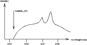
Figure 1.9
The continume is due to Bremsstrahlung radiation as accelerating charged particles emit radiation. Minumun wavelength l0 corresponds to all the electrons energy going into one photon of frequency f0 .
| eV0=hf0= |
|
(using equation 1.10, c=fl ) |
-
Characteristics
- line spectra depends on the target material. They were given arbitary names Ka, Kb ; La, Lb which in 1913 Moseley explained by applying Bohr's model to high Z atoms ( Z is the atomic number).
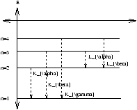
Figure 1.10
He realised that these short l , high energy photons result from electons dropping to the inner most energy levels as in figure 1.10.
We now know that in high Z atoms these levels are filled with electons, the Pauli exclusion principle prevents other electons joining them. The electon beam must first ionise an electon from the inner shell/level leaving a vacancy into which higher n electons fall and thus emitting X-Ray photons.
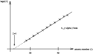
Figure 1.11
Mosely studied the characteristics of the spectrum. Plotting f against Z (the position in the periodic table) and observed
-
a better fit when f plotted against Z instead of atomic weight, concluding that Z was related to the nucleat charge (aka the number of protons).
- straight line passes through Z=1 and fitted by
f=a(z-1)2
(1.26)
where a=2.48× 10¹³ Hz
Mosely assumed Ka resulted from the electon dropping from n=2 to n=1 as in figure 1.10. He assumed that there were two electrons in the n=1 level. Before the n=2 electon can drip, one n=1 electon must be ionised. Therefore n=2 electon sees field of nucleus charge Ze and one electron, field due to charge (Z-1)e .
from equation 1.21
| E2-E1=hcRH(z-1)2 |
æ
ç
ç
è |
|
|
- |
|
) |
ö
÷
÷
ø |
=hcRH(z-1)2 |
æ
ç
ç
è |
|
|
- |
|
ö
÷
÷
ø |
=hf |
| Þ f= |
|
cRH(z-1)2=(2.47× 10¹⁵)(z-1)2 |
1.8 Compton Scattering
In 1923 Compton was studying X-ray scattering (l0=0.071nm) by relatively light atoms (Z=6, graphite) where the X-ray energy was 17.5keV which is much greater than the ionization energy. (by using equations 1.20 and 1.21, -E1=14.6Z2=490eV if Bohr applies).
On a classical picture he expected the charges in the atom to vibrate with the same f as the X-ray and re-emit with the same f . Indeed he observed scattered radiation with l0=0.071nm but he also observed X-rays at a longer wavelength l ' (as in figure 1.12) depended on the scattering angle but not on the target material.
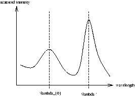
Figure 1.12
Compton explained the second peak by treaking the X-ray as a photon with energy Eg=pgc . This is what we expect relativistically for a zero mass particle given that
E2=p2c2+m2c4
(1.27)
and classically we know EM radiation exerts a pressure
| |
|
=P (eg. equation 33-29, p1039, Young |
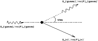
Figure 1.13
Momentum conservation in the lab
P1+P2=P3+P4
Energy conservation in the lab
E1+E2=E3+E4
The trick which helps solve equations 1.29 and 1.30 is to calculate an invariant quantity. eg. the rest energy of the recoil electron.
From equation 1.30
| |
( |
Ee' |
) |
|
= |
æ
è |
E |
|
+mec2-E |
|
ö
ø |
|
=E |
|
+me2c4+ |
æ
è |
E |
|
' |
ö
ø |
|
+2E |
|
mec2-2E |
|
E |
|
'-2E |
|
'mec2 |
| |
( |
Pe' |
) |
|
= |
æ
è |
P |
|
-P |
|
' |
ö
ø |
|
=P |
|
+ |
æ
è |
P |
|
' |
ö
ø |
|
-2P |
|
P |
|
' |
The invariant is:
| |
( |
Pe' |
) |
|
- |
( |
Pe' |
) |
|
c2=me2c4 |
| E |
|
E |
|
'-P |
|
P |
|
'c2=mec2 |
æ
è |
E |
|
-E |
|
' |
ö
ø |
| c2P |
|
P |
|
'=c2P |
|
P |
|
'cosq |
=E |
|
E |
|
'cosq |
| E |
|
E |
|
'-E |
|
E |
|
'cosq |
=E |
|
E |
|
'(1-cosq)=mec2 |
æ
è |
E |
|
-E |
|
' |
ö
ø |
| 1-cosq=mec |
æ
ç
ç
ç
è |
|
- |
|
ö
÷
÷
÷
ø |
=mec |
æ
ç
ç
è |
|
- |
|
ö
÷
÷
ø |
(by 1.28) |