

Chapter 3 Postulates of Quantum Mechanics
3.1 Operators and Eigenvalues
In section 2.5 wave functions which correspond to definate values of energy En were called energy eigenfunctions ( Un(x) ) and the En are energy eigenvalues.
Schrödinger's equation (equation 2.20) can be rewritten as
HUn(x)=EnUn(x)
(3.1)
This should remind you of the eigenvalue equation in Rowan Robinson's Maths Physics I course.
AU=lU
where:
-
U
- are eigenvectors
- l
- are eigenvalues
- A
- is a matrix
This is no coincidence, Heisenberg developed Quantum Mechanics comparable to Schrödinger's equation using matrices.
H is the total energy operator, or the Hamiltonia Operator
If we define a momentum operator
Operating twice with Px
therefore equation 3.2 can be written as
H is the none relativistic expression for the operator E with P2/2m replaced by an ?? (momentum)2/2m ??.
Let us operate with the momentum operator in equation 3.3 on the time independent travelling wave in equation ??2.19??.
|
HY(x)= h |
|
Y(x)=- |
|
Ae |
|
=- A( k)e |
|
= kAe |
|
= kY(x)
(3.4) |
Therefore we have Ae kx=Uk(x) a momentum eigenfunction which satifies the eigenvalue equation
PxUk(x)= kUk(x)=PxUk(x)
(3.5)
3.2 Postulates of Quantum Mechanics
Quantum Mechanics extended from observable quanties such as energy and momentum which had classical equilivents to other quanties such as angular momentum and spin some of which did not have a classical equilivent by assuming the following postulates:
3.2.1 Postulate I
With every physical obserable (ie. a measurable quantity) there is an associated operator Q . If Q is the operator associated with obserable q then measurement of q gives a result which is one of the eigenvalues of the equation
QUn=qnUn
(3.6)
Measurement must always give real numbers therefore the qn must be real. Mathematically the Q must be Hamiltonian. Two eigenvectors Um and Un of a Hamiltonian operator are orthogonal (ie. their eigenvalues are different). Handout 7 in Rowan Robinson's Maths Physics I course proved that
UnTUm=0 if qm qn
(3.7)
Equivelent to this if we know U(x) is the orthogonal relationship in equation ??2.29??
| |
ó
õ |
|
Um*(x)Un(x)dx=0 if m n |
3.2.2 Postulate II - Principle of Linear Superposition (Expansion Postulate)
The wave function of a particle represents everything which is know about the particle. Possible wave functions of a particle on a system can be expressed as a linear combination of the eigenfunctions or eigenvectors (eigenstates) of an operator.
The Cn are expansion co-efficients and thay can be complex in the general case.
3.2.3 Postulate III
The expectation value of an operator is the average of a large number of measurements identically prepared systems.
It can be shown (Problem Sheet 4, Q.4) that if the Un are normalised as in equation ??2.22?? and orthogonal as in equation ??2.29??
|
<Q |
>= |
|
|Cn|2qn= |
|
Pnqn
(3.10) |
It is only possibily to predict you will definitely get a result qn if the wave function equals Un
Y =Un
(3.11)
So if a measurement gives the result qn you know the wavefunction is as equation 3.11, so the measurement is repeatable (see Classwork 5). In all other cases one can only deal with probabilities that you will get a certain result as in equations 3.9 and 3.10.
3.3 Examples if the Use of Our Quantum Mechanic Postulates
3.3.1 The Vector Analogy
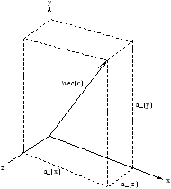
Figure 3.1
The right hand side of the equation is made up from eigenfunctions and eigenvectors.
The wave function is equilivent to a vector in three dimensional space as in figure 3.1. Any r vector in any direction can be represented by different expansion co-efficients ax , ay and az . Note that x , y and z are othogonal and normalised to untity as for Un .
To find ay (for example)
y.r=0+ayy.y+0=ay
In Quantum Mechanics to find a particular Cm you take
As long as the Um values are orthogonal and normalised.
Only if ay=1 and ax=az=0 can you be sure that r is pointing in the direction y .
3.3.2 Zero Point Energy
An electron in an infinite potential well as in section 2.5. Assume we have measured the energy and have found the result E1 . Quantum Mechanics says we have operated with the H and found the energy eigenvalue from equation ??2.27??.
The only way we can be sure we have this result is if the Y of the electron is the corresponding eigenfunction by equation 3.11.
| Y =U1=Asin |
|
(from equation ??2.28??) |
3.3.3 Quantum Mechanical Bonding
THIS SUBSECTION IS NOT EXAMINABLE
The principles of quantum mechanical bonding, fundamental to Chemistry and Solid State Physics, can be understood on the basis of the Superposition Principle without getting tied-up in the mathematics. The procedure is an example of Perburbatian Theory and many are put off by its mathematical nature. Feynman Volume III, Chapter 9, 10 and 13 gives a very logical presentation of the maths.
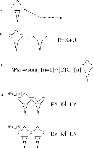
Figure 3.2
-
Figure 3.2a
- represents the assumption that we have solved Schrödinger's Equation for a 1 Datom, we know the energy levels and the wave function of the outer electron.
- Figure 3.2b
- represents the wish to know what happens if we bring up from infinity an identical atom without its outer electron.
- Figure 3.2c
- represents the fact that, according to Superposition, the general solution to (b) is the sum of solutions to (a) with the one electron on each atom.
- Figure 3.2d
- represents the two solutions with definite energy for the (electron and two atoms) system.
-
The Antisymmetric YA
- has higher E that (b) (atoms seperated)
-
Potential Energy
- is lower because the electron is lower in the wells ( Y =0 at midpoint)
- Kinetic Energy
- is higher because electon more confined ( (D Px)2 higher)
- The Symmetric YS
- has lower E than (b)
-
Potential Energy
- is higher because the electron is more likely to be out of the wells
- Kinetic Energy
- is lower because YS more spread, therefore (D Px)2 is smaller
Note that the Uncertainity Principle effect of kinetic energy is more than the potential energy shape effect. If you bring up the second well, electron can minimise its potential energy by spreading time in both wells without the kinetic energy penalty of cenfiniment into one well. Hence two identical atoms plus one electron have lower E than one electron plus seperate atoms.
A Similar Argument
One electron plus three identical, equally spaced atoms will have three total energy eigenstates, one of which will have lower total energy than one electron plus three seperate atoms.
One electron plus n identical, equally spaced atoms will have n total energy eigenstates, the lowest of which will have lower total energy than one electron plus n seperate atoms.
These n closely spaced energy levels is the conduction bond. This nearly free electron helps to bind the solid. The electron on the first atom is not in one of these n total energy eigenstates. The coupled oscillator analogy suggests the electron will therefore propagate down the line. This ecplains how an electron in a crystal with spacing a0 can have l>100a0 (Structure or Matter, Problem Sheet 5, Q3).