Chapter 1   Maxwell's Equations

1.1   Electric Charge

• positive and negative charges exists. Their value's match to at least one part in 10²⁰ . The smallest amount of (stable) charge you can have is 1.6022× 10^-19 C
• charge is conserved
• charge is invarient under Lorentz Transformation
• the force between two charges obeys Coulomb's law
  
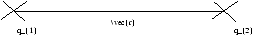
  Figure 1.1 - Force Between Two Charges

  F=

  q1q2 4pe0

  r r2

  where e₀=8.85× 10^-12 Fm^-1 and r=r/|r| which is the unit vector of r .
• comparing the Coulomb force between two electrons with the gravitational force setup between them

  Fc=

  e2 4pe0r2

  ,  Fg=

  GMe2 r2

  the ratio of the two forces

  Fg Fc

  =10-42

  although this is a very small value gravity still matters as on large scales the number of positive and negative charges are more or less equal.
• moving charges produce another force, the magnetic force

1.2   Magnetism

1.3   Vector and Vector Fields

1.4   Revision of Maxwell's Equations

• E is the electric field vector and its units are in volts per metre
• B is the magnetic field vector and measured in tesla's
• r is the total charge density and is measured in coulombs per m³
• the total current density ( j ) is measured in amp's per m²

1.4.1   Electric Field

charges (coulomb's law):

the electric field of a stationary charge q at a distance r is

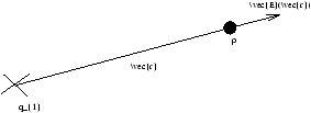
Figure 1.2 - Coulomb's Law for a Point Charge

E=

q rpe0

r r2

Vm-1     (1.1)

however this only for a point charge, for a non-point charge we need to integrate equation 1.1 over a surface S which is enclosing the charge

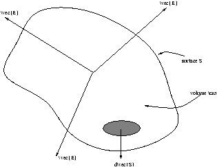
Figure 1.3 - Coulomb's Law for a Non-Point Charge

for a spherical surface (which is then true for any surface)

S

E.dS=

q e0

for many charges within the surface S

S

E.dS=

1 e0

å i

qi

where q_i is the i^th charge. For a distributed charge density r(r)

S

S.dS=

1 e0

ó õ

t

r dt     (1.2)

this is Gauss' Law. If we use divergence theorem we obtain

ó õ

t

æ ç ç è

Ñ .E-

r e0

ö ÷ ÷ ø

dt =0

so

Ñ .E=

r e0

(1.3)

this is Maxwell's First Equation

electromagnetic induction:

we define the electromotive force

=

C

E.dl volts

where C is the line integral around the circle l

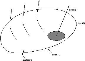
Figure 1.4 - Magnetic Induction

we now assume there is a magnetic field through the circuit and so we define flux ( F ) associated with B as

F =

ó õ

S

B.dS Webers

Faraday's Law is

C

=E.dl= =-

¶F ¶ t

(1.4)

Stokes :aw gives use

ó õ

S

(Ñ×E).dS=-

¶ ¶ t

ó õ

S

B.dS

Ñ×E=-

¶B ¶ t

(1.5)

1.4.2   Magnetic Field

no magnetic charges:

it can be shown from Bio-Savart that

Ñ .B=0     (1.6)

which is Maxwell's Third Equation. By using the divergence theorem we obtain

B.dS=0     (1.7)

magnetic field's due to currents:

steady current:

the Biot-Savart Law (1820) says

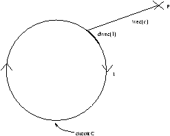
Figure 1.5 - Steady Current

the magnetic field at P a distance r from a circuit is

B=

µ0I 4p

C

dl×r r2

Telsa

where µ₀=4p× 10^-7 Hm^-1 and is called the permability of free space

generalise:

we consider the current density j Am^-1 in a volume t

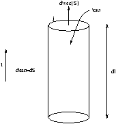
Figure 1.6 - Generalising the Biot-Savart Law

then

Idl=jdSdlj=jdt

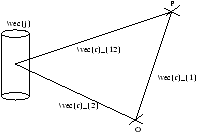
Figure 1.7 - ???

B

=

ó õ

all space

µ0 4p

j(r2)×r12 |r12|2

dt     (1.8)

we take the curl of equation 1.9 and obtain the Bio-Savart Law

Ñ×B=µ₀j     (1.9)

or

C

B.dl=µ0I

this is the steady current law (Ampere's Law). However this is incomplete. So by taking the divergence of equation 1.10

Ñ .(Ñ×B)=0µ₀Ñ .j

we require that there is charge gain or loss from the body

Ñ .j=-

¶r ¶ t

(1.10)

and integral form

S

j.dS=-

¶ ¶ t

ó õ

t

r dt

displacement current:

we use equation 1.1 to write

r =e₀Ñ .E

and this is substituted into equation 1.11

Ñ.

é ê ê ë

j+e0

¶ E ¶ t

ù ú ú û

=0

If the j in the Maxwell Equation (equation 1.10) with

j+e0

¶E ¶ t

we obtain

Ñ×B=µ0j+µ0e0

¶E ¶ t

(1.11)

this is Maxwell's Forth Equation, or it can be written as

C

B.dl=µ0I+µ0e0

¶ ¶ t

FE     (1.12)

FE=

ó õ

S

E.dS

1.4.3   Internal Consistency

1.4.4   Force of Particle

1.5   Materials in Electromagnetic Theory

conductors:

are an assembly of microscopic charged particles which are free to move about. For example conduction bands with electrons and also Ions are proportional to electrons in a plasma.

Figure 1.8 - A Conductor

we make the following definitions

free charge density ( r_f ):

this is the charge density in the conductor

conduction current density ( j_f ):

is the density of the current in a conductor

dielectrics:

are an assembly of microscopic electic dipoles. For example the number of equal charges is proportional to the number of opposite charges where q is separated by a distance l

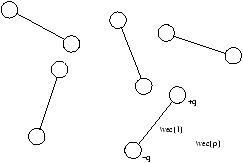
Figure 1.9 - A Dielectric

we make the following definitions

the dipole moment ( p ):

p=ql Cm

electric polarisations ( P ):

P=å_tp/t Cm^-2
This is a macroscopic quantity where t is the volume. P is a flux of charge out of the volume t

polarisation charge density ( r_P ):

by considering a volume t bounded by a surface S

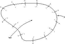
Figure 1.10 - Polarisation Charge Density

if we consider all the dipoles to be pointing outwards and so the volume is negatively charged we can calculate r_P Cm^-3 . To relate r_P to vecP , the net charge due to polarisation is

dQ_P=-P.dS

if this is integrated

QP=-

S

P.dS

and then by using the divergence theorem

QP=-

ó õ

t

Ñ .Pdt

also

QP=

ó õrPdt

this can be equated to obtain

r_P=-Ñ .P

polarisation current density ( j_P ):

states that charge is to be conserved

-

¶rP ¶ t

=Ñ .jP

we have r_P=-Ñ .P which we can substitute to obtain

jP=

¶P ¶ t

(1.14)

so we finish of with the current being

j=jf+

¶P ¶ t

+

and the charge to be

r =r_f-Ñ .P+0

where

magnetic:

are an assembly of microscopic magnetic dipoles formde from current loops.

Figure 1.11 - Magnetic Materials

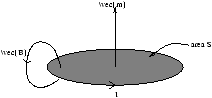
Figure 1.12 - A Current Loop

we define

dipole moment:

m=IS Am²

magnetisation:

M=å_tm/t Am^-1

magnetic charge density:

is zero

magnetisation current density ( j_m ):

is the current density associated with the current loops

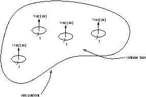
Figure 1.13 - Dipoles Summing to a Current

we recall that Ñ .B=µ₀j for the total j so we can define

j_m=Ñ×M     (1.15)

The proof is tedious and so overlooked (see First Year EM Notes for Dr. Coppin's Lectures)

1.6   Forms of Maxwell's Equations

1.6.1   Second Universally Valid Form of Maxwell's Equations

Gauss' Law:

Ñ .E=

r e0

=

1 e0

(rf-Ñ .P)

or

Ñ .(e₀E+P)=r_f

we define the electric displacement

D=e₀E+P

so we can rewrite Gauss' Law as

Ñ .D=r_f     (1.18)

Amperes-Maxwell Equation:

Ñ×B=µ0j+µ0e0

¶E ¶ t

Ñ×B=µ0

é ê ê ë

jf+

¶P ¶ t

+Ñ×M

ù ú ú û

+µ0e0

¶E ¶ t

Ñ×

æ ç ç è

B µ0

-M

ö ÷ ÷ ø

=jf+

¶D ¶ t

we define H=B/µ₀-M as the magnetic field vector, this gives us

Ñ×H=jf+

¶D ¶ t

(1.19)

1.6.2   Maxwell's Equations in a Homogeneous Isotropic and Linear Medium (A HIL Medium)

homogeneous (H):

means the same at all points in space

isotropic (I):

means it responds the same in every direction

linear (L):

PµE and MµH

1.7   Vector and Scaler Potentials

1.7.1   The Scaler Potential (Feymann, Chapter 6)

1.7.2   The Vector Potential (Feymann, Chapter 14, 15 and 18)

1.7.3   Generation of Electromagnetic Radiation

1.8   Electromagnetic and Special Relativity

1.8.1   The Lorentz Transformation of Electromagnetic Fields

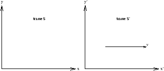
Figure 1.14 - The Lorentz Transformations

in frame S:

E=0 and V=By

in frame S':

E_z'=g vB and B_y'=g B_y

1.8.2   Four Vectors (Feymann, Chapter 25)