


Chapter 2 Theory of Gases
2.1 Ideal Gas Law
Observational Evidence (note that this is only true at low densities):
-
Pressure is inversely proportional to volume (Boyle's Law - 1662)
- At fixed volume, pressure is proportional to temperature (Charles and Gay-Lussac Law - 1800)
pµ T
- At fixed pressure and temperature, the volume of a gas is proportional to the total number of molucules
Vµ N
Therefore we can conclude
pVµ NT Þ pV=kBNT
where kB is Boltzmann's constant ( kB=1.381× 10⁻²³ JK-1 ).
2.2 Definitions
2.2.1 The Mole
Due to the large numbers involved, in practical situations it is convenient to define a new unit of quantity.
One mole is defined as the number of atoms in twelve grammes of C612 . This quantity is called Avogadro's Number.
NA=6.022× 10²³
Number of moles is equal to the number of molecules divided by Avogadro's Number.
substitute for N in the ideal gas law equation
pV=nmNAkBT Þ pV=nRT
where R=NAkB=8.314 Jmol-1K-1 (the universal gas constant).
2.2.2 Atomic Masses
Mass of NA atoms of C612=12g (by definition).
Mass of one atom of C612=12/NAg .
But one atom of C612 has mass of twelve atomic mass units (amu).
| 1 amu= |
|
g= |
|
kg=1.66× 10⁻²⁷ kg |
A molecule with molecular mass M amu will have mass m=M/NAg .
2.2.3 Density of Gas
substitute into the ideal gas law
Þ pM=r RT
2.3 Kinetic Theory of Gases
Relationship between microscopic properties and macroscopic state of an ideal gas.
Assumptions:
-
contains a large number of identical molecules
- molecules are small, hard spheres in constant random motion
- molecules collide perfectly elastically with each other and with the walls of the container
- walls are perfectly rigid and infinitely massive
- no intermolecular forces
Speed v can be resolved into three orthogonal components; Vx , Vy and Vz such that
V2=Vx2+Vy2+Vz2
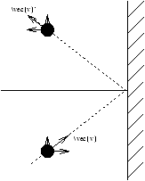
Figure 2.1 - Collision on a Single Particle
Perfectly elastic collision so
V'x=-Vx; V'y=Vy; V'z=Vz=0
V'2=V2
Initial momentum x direction
Px=mVx
Find momentum
P'x=mV'x=-mVx
change in momentum is
D Px=P'x-Px=-2mVx
Newton's II: F=dP/dt
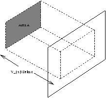
Figure 2.2 - All molecules in the box length
VxD t will hit the wall within time
D t
Number of molecules per unit volume
Number of molecules in the box is N/VAVxD t . Only half of these molecules are traveling in the positive x direction so the number of molecules hitting the area A in time D t is 1/2×N/VAVxD t .
Change in momentum is -2mVx×1/2×N/VAVxD t .
2.4 Temperature and Kinetic Energy
Kinetic theory is only consistant with ideal gas laws
The average tr/anslational kinetic energy of a molecule is
so for one molecule Þ =3/2KtrT
so for one mole Þ Ktr=3/2RT
Absolute temperature is a measure of the average translational kinetic energy of the molecules in an ideal gas. Note that Ktr depends only on T .
From the above equation we can deduce the root-mean-square speed of the molecules from the temperature
2.5 Specific Heat Capacities of Gases
Heat is the energy that is transfered between two bodies because they are at different temperature (see section 6).
If addition of a quantity of heat D Q raises the temperature of a substance of mass M by D T then the specific heat, c is defined by:
D Q=cMD T
c=Jkg-1K-1
Molar specific heat, C is defined by
D Q=CnmD T
C=Jmol-1K-1
The amount of heat required will actually depend on the conditions imposed during the heating.. If the volume is kept fixed the specific heat is Cv , otherwise if the gas is allowed to expand then more heat will be required to raise the temperature by 1K . So if the pressure is kept constant the specific heat is Cp .
If the temperature changes by D T then kinetic energy will change by
If the only energy possessed by the gas is in translational kinetic energy then DKtr=D Q .
From comparison of Ktr=3/2nmRT at constant volume Cv=3/2R . (see table 16-1 in Young and Freedman).
-
Diatomic
-
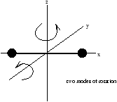
Figure 2.3 - About the x-axis the moment of inertia is negligible
- Triatomic (and more)
-
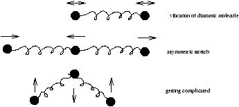
Figure 2.4 - Molecular Vibrations Become Complicated
So for the specific heat values, they are different due to vibration and rotation of the atoms in the gas for diatomic/triatomic/polytomic.
For diatomic molecular vibration occurs along the axis. For polyatomic molecules there may be many modes of vibratin. Can we predict the specific heat capacities of diatomic and polyatomic gases? Yes!
2.6 Equipartition of Energy
Each defree of freedom has an average energy of 1/2RT per mole.
The number of degrees of freedom is the number of terms in the expression for the total energy which form a quadratic in an independent dynamical variable (eg. velocity, position, angular momentum, etc).
| Ktr= |
|
mvx2+ |
|
mvy2+ |
|
mvz2 per molecule |
| E= |
|
RT (from Equipartition of Energy) |
Erot=Iw2=Ixwx2+Iywy2+Izwz2 per molecule
for a diatomic molecule lying along the x-axis, Ix is small so we can conclude that there are only two rotational degrees of freedom. Therefore for diatomic molecules (no vibrational energy) there are three translational and two rotational degrees of freedom leading us to a total of five degrees of freedom.
Considering the vibrational energy we can model the molecule bonds as springs where the potential energy is 1/2kx2 where k is the spring constant. The kinetic energy for this situation is 1/2mvx2 . Therefore for a diatomic molecule there are another two degrees of freedom due to the vibrational energy of the molecule, so Cv=7/2R .
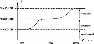
Figure 2.5 - The Specific Heat at a Constant Volume for
H2
Figure 2.5 shows that some of the degrees of freedom do not become active until higher temperatures are reached, therefore we can conclude that Cv is a function of T .
For polyatomic molecules the rotational and vibrational energies can be excited at a much lower temperature than it is for H2 .
2.7 Real Gases
Ideal gases obey Boyles Law
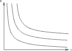
Figure 2.6 - Boyles Law (
pµ1/
V ) for an Ideal Gas (with lines of isotherms)
however for real gases we get a different situation
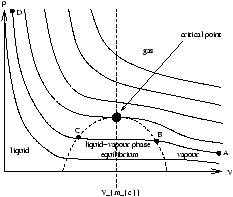
Figure 2.7 - A Real Gas (with lines of isotherms)
Figure 2.7 is a p-V diagram shoing the isoterms for the gas and liquid-vapour phases and also the critical point and isotherm at the critical temperature Tc .
At high temperatures the gas more or less behaves as an ideal gas, however at low temperatures (or high densities due to a small Vm ) the gas behaviour deviates from the ideal. Consider the isothermic compression of the gas along the route A-B-C-D.
-
A ® B:
- p rises approximately in accordance with Boyle's Law
- B ® C:
- further compression causes the gas to liquify providing a sharp drop in Vm at a constant temperature
- at C:
- the gas has been liquified and a further increase in p results in only a small decrease in Vm (C ® D) because liquid is more or less uncompressible
- at T>TC :
- the gas constant cannot be liquified by isothermal compression. We define a vapour as a gas at T<TC which can be liquified by isothermal compression
The breakdown of the ideal gas law occurs because we have negleted the finite size of the molecules and the attractive forces between them.
2.7.1 Van der Waal's Equation
Van der Waal's equation of state is based on measured values for p and Vm .
a and b are constants, different for each gas, that are derived from measurements.
A comparison of this with the Ideal Gas Law (section 2.2.2) we define
otherwise written as
The measured value of p is less than that which would be measured in an ideal gas because of the attractive force between molecules. The pressure on the wall of the container is reduced by the force of attraction by the molecules in the body of the gas.
The attractive force on one molecule is directly proportional to the pressure however he number of molecules hitting the wall is also directly proprortional to the pressure. Therefore the total reduction in pressure is proportional to p2 (or proportional to 1/V2 ). Hence this gives us
We now define VmIG=Vm-b as what is observed from experiment is
The measured value of Vm is greater than the ideal gas molar volume due to the space occupied by the molecules them selves. However we note that for large Vm the Van der Waal equation tends to the Ideal Gas Law.
2.8 Probability Distribution
So far in discussing the speeds and kinetic energies of molecules we have only considered the average quantities Ktr and v (sections 2.3 and 2.5). In fact molecules will have a distribution of energies and speeds.
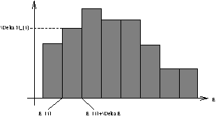
Figure 2.8 - Distribution of Molecular Energies in Finite Intervals
The two constraints on the histogram are
-
the total number of molecules is N
åD Ni=N
- if the mean energy is E then
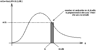
Figure 2.9 - Energy Distribution
For infinitessimal values of dE the energy histogram becomes the Energy Distribution
however again there are two constraints on the distribution
-
ò0¥n(E)dE=N
- 1/Nò0¥En(E)dE=E
the probability distribution is
this would give the probability of a molecule having a certain energy level, so another constraint is
2.9 Density of States
In order to predict the energy distribution we need to know the possible energy states a molecule might occupy. A single energy level (ie. value) may correspond to more than one energy state in which case the level is said to be degenerate.
for example, suppose that 2E/m=50 , this implies that there are many ways to make up the energy level, however each different combination is a different state.
In classical physics it is difficult to count energy states because the speed, and thus the energy, values can be arbitrary close together resulting in an infinite number. In Quantum Mechanics the number of states is restricted because only certain states are allowed.
Never-the-less we can assess the relative number of energy states by considering their distribution in velocity space.
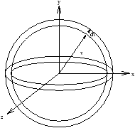
Figure 2.10 - Number of States in (
E,
E+
dE) or (
v,
v+
dv)
If the states are uniformly distributed in velocity space then the number in (E,E+dE) is proportional to the volume of the spherical shell which is 4p v2dv . However E=1/2mv2 therefore dE=mvdv and so we obtain dv=dE/mv . Therefore the number within the shell is
the density of states is the number of states per unit energy interval
2.10 Density of States in Two Dimensionals
SEE CLASSWORK SHEET TWO
2.11 Distribution of Molecular Energies
We want to know the number of molecules per unit energy. Interval N is large so the number of molecules in a particular level will be determined statistically by the probability of a molecule having that energy.
Thus we need to know the number of ways of putting N molecules into the energy levels Ei , each of which has gi possible states, such that the total energy is
Etotal=NE
2.11.1 An Example
Lets consider that
N=3, Etotal=4
where the energy levels are integers with g(0)=1 , g(1)=2 , g(2)=3 , g(3)=3 and g(4)=4 ; these are linked together by the relationship 2E1/2 . Combinations of three molecules such that the total energy level is four can be made up in the following four combinations:
| E |
A |
B |
C |
D |
| 4 |
1 |
0 |
0 |
0 |
| 3 |
0 |
1 |
0 |
0 |
| 2 |
0 |
0 |
2 |
1 |
| 1 |
0 |
1 |
0 |
2 |
| 0 |
2 |
1 |
1 |
0 |
| |
however if the molecules are distinguishable
-
A:
- has three combinations
- B:
- has six combinations
- C:
- has three combinations
- D:
- has three combinations
the energy levels are degenerate so that a molecule in level four can be in any of the g(4)=4 states.
2.11.2 Consider the Effect of Density of States
For each of the arrangements in combination A there are g(4)g(0)g(0)=4 possibilities which is 4× 1× 1=4 . So the total number of possibilities under combination A is
(possibilities per molecule)× (number of arrangements)=(total)
4× 3=12
for the combination B each arrangement has g(3)g(1)g(0)=6 possibilities so the total number of possibilities fo B is
6× 6=36
If we continue this we find there are a grand total of 111 possibilities. So the average number of molecules in level four is
these values sum to three as there are three molecules present.
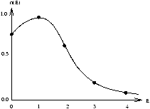
Figure 2.11 - ???
from figure 2.11 we can conclude that
| E |
n(E) |
g(E) |
f(E) |
| 4 |
0.11 |
4 |
0.03 |
| 3 |
0.32 |
3 |
0.11 |
| 2 |
0.81 |
3 |
0.27 |
| 1 |
0.97 |
2 |
0.49 |
| 0 |
0.78 |
1 |
0.78 |
| |
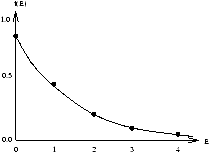
Figure 2.12 - ???
f(E) looks like a proportional to e-aE . Is this true? YES! Statistical Mechanics shows the general result
however we note that for an ideal gas g(E)µ E1/2 so
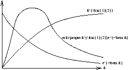
Figure 2.13 - Energy Distribution for Three Dimensional Gases
what are the constants?
we find the constants A and b by using the constrants listed in section 2.8:
-
by using the standard integral
we obtain
-
by using the standard integral
we obtain
| |
æ
ç
ç
è |
|
ö
÷
÷
ø |
æ
ç
ç
è |
|
ö
÷
÷
ø |
æ
ç
ç
è |
|
ö
÷
÷
ø |
|
=E |
we now solve these equations simultaineously
this is the Ideal Gas Law, we now substitute for b into the first equation
| Þ n(E)=2p N |
æ
ç
ç
è |
|
ö
÷
÷
ø |
|
E |
|
e |
|
n(E)µ g(E)fMB(E)
The most probable energy Emp is where n(E) is a maximum
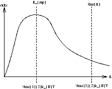
Figure 2.14 - The Most Probable and Mean Energy
2.12 Distribution of Molecular Speeds
n(v)dv=n(E)dE
as we know that E=1/2mv2
| n(v)=n(E) |
|
=2p N |
æ
ç
ç
è |
|
ö
÷
÷
ø |
|
E |
|
e |
|
mv |
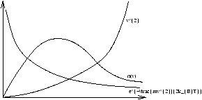
Figure 2.15 - Speed Distribution for Three Dimensional Gases
the mean speed is
| v |
=B |
ó
õ |
v3e |
|
dv, Bº 4p |
æ
ç
ç
è |
|
ö
÷
÷
ø |
|
| Þ v |
=- |
ó
õ |
|
- |
|
e |
|
2vdv=B |
|
é
ê
ê
ê
ë |
- |
|
e |
|
ù
ú
ú
ú
û |
|
=2B |
æ
ç
ç
è |
|
ö
÷
÷
ø |
|
= |
æ
ç
ç
è |
|
ö
÷
÷
ø |
|
| vrms=(v |
2) |
|
= |
æ
ç
ç
è |
|
ö
÷
÷
ø |
|
= |
æ
ç
ç
è |
|
ö
÷
÷
ø |
|
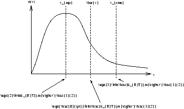
Figure 2.16 - ???