Chapter 3 Series Solutions of Differential Equations
3.1 Introduction
These are functions defined by series such as
-
finite series:
-
- infinite series:
-
-
y=a0+a1x+a22+a3x3+...
- eg. sinx=x-x3/3!+x5/5!+...
- The Taylor Series
| f(x)=f(a)+f'(a)(x-a)+f''(a) |
|
+f'''(a) |
|
+... |
- The Maclarine Expansion (the Taylor Series where a=0 ), for example
-
(1+x)1/"=1+x/2-x2/8+x3/16-5x4/128+...
- 1/1-x=1+x+x2+x3+x4+...
- cosx=1-x2/2!+x4/4!+...
- ex=1+x/1!+x2/2!+x3/3!+... (for all x )
We could consider the functions (eg. sinx , cosx , ex , ...) as being defined as the solutions to particular differential equations.
To demonstrate this we will seek series solutions to the linear second order different equation
we already know thought that the solutions are sinx and cosx however this helps us to understand this technique of using power series to obtain our solutions.
We assume that the solution(s) are given by
how are we to find the values of an ?
y=a0+a1x+a2x2+a3x3+a4x4+...+anxn
we need to differentate this twice
| Þ |
|
=0+0+(2.1.a2)+(3.2.a3x)+(4.3.a4x2)+...+((n+2)(n+1)an+2xn |
| |
|
+y= |
|
[ |
(a+2)(n+1)an+2+an |
] |
xn=0 |
For this to hold for all x the coefficient of xn must be zero for all n .
-
even n :
-
-
n=0 2.1.a2=-a0
- n=2 4.3.a4=-a2
- n=4 6.5.a6=-a4
- odd n :
-
-
n=1 3.2.a3=-a1
- n=3 5.4.a5=-a3
- n=5 7.6.a7=-a5
this can be reduced to
-
even n :
-
-
2!a2=-a0
- 4!a4=(-1)2a0
- 6!a6=(-1)3a0
- odd n :
-
-
3!a3=-a1
- 5!a5=(-1)2a1
- 7!a7=(-1)3a1
you will notice that the odd values are not related to the even values, we can already see two solutions emerging.
The general pattern for the even values of n is
The general pattern for the odd values of n is
Note that the general solutions contain no relation between a0 and a1 .
| Þ y=a0 |
é
ê
ê
ë |
1- |
|
+ |
|
- |
|
+... |
ù
ú
ú
û |
+a1 |
é
ê
ê
ë |
x- |
|
+ |
|
- |
|
+... |
ù
ú
ú
û |
From the knowledge of our Maclarine Expansion's we deduce
y=a0cosx+a1sinx
where a0 and a1 are arbitrary constants.
Note that we will see later that we will have to consider anxn where n is not a positive integer.
3.2 Some of The Differential Equations Of Mathematical Physics - 2 Dimesions
Examples of these types of equations are
-
Helmhotz's Equation:
- Ñ2u+l u=0
- Poussin's Equation:
- Ñ2u=f(x,y,z)
- Schrödinger's Equation (time independent):
- Ñ2+a (E-V(x,y,z)u)=0
- Schrödinger's Equation (time dependent):
- ¶ u/¶ t=-2/2m¶2u/¶ x2+V(x)u
- Telegraph Equation:
- ¶2u/¶ x2-¶2/¶ t2-¶ u/¶ t=0
- Fokker Planck Equation:
- ¶ u/¶ t=a¶2/¶ x2+b¶ (x,y)/¶ x
3.2.1 The Wave Equation
Summary
recalling that
normally we would have to consider in real life applications that u=u(x,y,z,t)
however we will really only consider two variable equations, for example
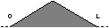
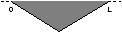
Deriving - Wave on a String
Lets consider a wave on a string in one dimension
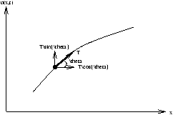
Figure 3.1 - Wave on a String
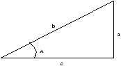
The transverse force is Tsinq which we can approximate to Tq for small q . We also have tanq=¶ u/¶ x~q , again for small q .
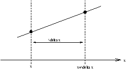
Figure 3.2 - Considering a Small Section of the String
| F(x+d x)=F(x)+T |
|
æ
ç
ç
è |
|
ö
÷
÷
ø |
d x+... |
An Extra Note on Waves on a String (stretched)
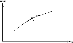
Figure 3.3 - The Tension (
T ) in a String
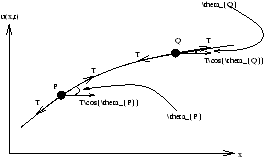
Figure 3.4 - The Components of Tension in the String
This is true for when qP and qQ are small and also when qP¹qQ
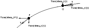
Figure 3.5 - Some on the Tension Components Cancel
this is because TcosqP~ TcosqQ~ T
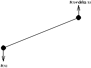
Figure 3.6 - When the String is Cut
When the string is cut we get an acceleration occuring and so
r dx=mass
Deriving - Maxwell's Equation
D=ere0E, B=µrµ0H
in an non-conductor r=0 and J=0
Ñn(ÑnE)=Ñ(Ñ.E)-Ñ2E-Ñ2E
as Ñ(Ñ.E)=0 we get
| -Ñ n |
æ
ç
ç
è |
|
ö
÷
÷
ø |
=-µrµ0 |
æ
ç
ç
è |
Ñn |
|
ö
÷
÷
ø |
=-µrµ0 |
|
=-µrµ0ere0 |
|
=-Ñ2E |
3.2.2 (Heat) Diffusion Equation
Summary
Deriving
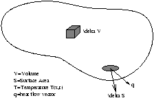
Figure 3.7 - Heat Dispersion
The heat contained in the volume d v is
d h=T(r,t)r(r)c(r)d v
where r(r) is the density and c(r) is the heat capacity.
Therefore the total heat contained is
| H= |
ó
õó
õó
õ |
|
T(r,t)r(r)c(r)dv |
| |
|
=- |
ó
õó
õ |
|
q.ds |
=- |
ó
õó
õó
õ |
|
dwqdv |
| |
|
= |
|
é
ê
ê
ê
ê
ë |
ó
õó
õó
õ |
|
T(r,t)r(r)c(r)dv |
ù
ú
ú
ú
ú
û |
= |
ó
õó
õó
õ |
|
r(r)c(r) |
|
dv |
| |
ó
õó
õó
õ |
|
r(r)c(r) |
|
[T(r |
,t)]dv=- |
ó
õó
õó
õ |
|
Ñ .q dv |
| |
ó
õó
õó
õ |
|
æ
ç
ç
è |
r (r)c(r) |
|
+Ñ.q |
ö
÷
÷
ø |
dv=0 |
We now assume that
q-KÑT
where the minus sign is as heat transfer is from hot to cold and the K is the conductivity of the volume.
so for any subvolume
3.2.3 Laplace's Equation
Summary
Deriving
Thus
Ñ.Ñf =0
Ñ2f =0
and in a two dimensional system
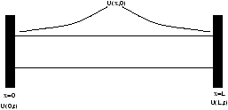
Figure 3.8 - We Need An Initial Condition (for example
U(
X,0) )
An Example of the boundary conditions we can use, in this case for Laplaces Equation
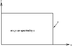
Figure 3.9 - Boundary Conditions for Laplaces Equation
or we could
Figure 3.10 - A Different Boundary Condition
where the normal boundary condition is ¶ u(x,y)/¶ n
3.2.4 A Note About Boundary Conditions and Initial Conditions
The wave and heat equations depend upon time so we expect to have to specify some initial conditions.
For the Wave, Heat and Laplaces equations, all of which depend upon space coordinates and so we have to specify conditions of spatial boundary.
Example - A Wave on a String
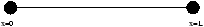
Figure 3.11 - A Wave on a String
Usually from here we would specify the shape of the sting at t=0
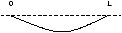
u(x,0)=f(x) (0£ x£ L)
also we could specify the strings velocity at t=0
note that if g(x)=0 then the string is stationary at t=0 .
These are conditions of general boundary conditions. For spatial conditions we have
-
fixed ends:
-
-
u(0,t)=0 for all t
- u(L,t)=0 for all t
these are homogenous boundary conditions
- sliding fixture:
- an alternative type of boundary condition can be the sliding fixture
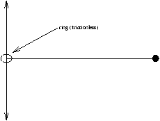
Figure 3.12 - The Sliding Fixture Boundary Conditions
so the boundary condition becomes
For all these specifications we would need four boundary conditions as we have a pair of second order differential equations. What we choose as the specification is up to us and makes no difference.
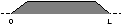
Example - The Heat Equation
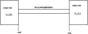
Figure 3.13 - A Thin Insulated Rod
u(0,t)=U0; u(L,t)=UL
Other examples of the heat equation and possible boundary conditions are:
-
Particle/Dye Diffusion Uses Same Heat Equation:
-
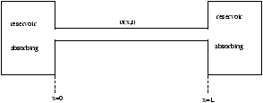
Figure 3.14 - Particle/Dye Diffusion
u(0,t)=0; u(L,t)=0
these are known as absorbing boundary conditions
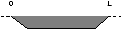
- Thin Insulated Rod With Insulators at Either End:
-
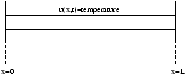
Figure 3.15 - Thin Insulated Rod With Insulators at Either End
there is no heat transfer across the insulator boundaries, there are called reflective boundaries
- Partial Boundaries (aka Partial Reflective):
-
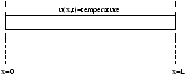
Figure 3.16 - Thin Insulated Rod With Partial Boundaries
3.3 Method of Seperation of Variables
This can be applied to linear homogenous equations. The technique is quite general, we follow two steps
-
seperate the variables, this produces a differential equation of some order that needs solving.
- apply the boundary conditions
3.3.1 An Example
where u=u(x,t) . We assume that we can obtain a solutions of the form
u(x,t)=X(x)T(t)
we now subsitute into the partial differential equation
so
we now divide by u(x,y)=X(x)T(t)
we now have seperated the indepedent variables x and t . So this equation must hold for all values of x and t .
Suppose we choose a particular value of x then the left hand side takes on a value and the right hand side has to equal this value for all t . So for example the left hand side is equal to the right hand side which equals a constant.
More formally if we look at
and this is true of the vice versa
now we let the left hand side to equal the right hand side to both equal a seperation constant. We will see later that we need to distinguish between the constant being zero, positive or negative. So we choose the constant to be either 0 , -k2 or +k2 .
We now put the seperation constant to equal:
-
zero:
-
Þ X=Ax+B, T=Ct+D
where A , B , C and D are constants.
u(x,t)=(Ax+B)(Ct+D)
- -k2 :
-
X''+k2X=0
X=Acos(kx)+Bsin(kx)
this solution looks like a solution to simple harmonic motion
so also
T''+k2c2T=0
T=Ccos(kct)+Bsin(kct)
- +k2 :
-
X''-k2X=0
we now try X=emx
(m2-k2)emx=0
m2=k2
Þ m=± k
X=Aekx+Be-kx
this solution does not look like a wave like solution.
so also
T''-k2c2T=0
T=Aekct+Be-kct
however this can be re-written as
ex=coshx+sinhx, e-x=coshx-sinhx
by using these we can obtain
X=A'cosh(kx)+B'sinh(kx)
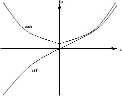
Figure 3.17 - A Plot of
X=
A'cosh(
kx)+
B'sinh(
kx)
Now we have the following solutions
-
type 1 ( k=0 ):
- u(x,t)=(Ax+B)(Ct+D)
- type 2 ( -k2 ):
- u(x,t)=(Acos(kx)+Bsin(kx))(Ccos(kct)+Dsin(kct))
- type 3 ( +k2 ):
- u(x,t)=(Acosh(kx)+Bsinh(kx))(Ccosh(kct)+Dsinh(kct))
Note that to proceed any further we need to apply boundary (or initial) conditions. Also a boundary condition is said to be homogenous if all terms contain u or ¶ u/¶ x , etc.
eg. u=0 is a homogenous boundary condition.
¶ u/¶ x=0 is also homogenous.
u(x,0)=f(x) is not homogenous, this is known as inhomogenous.
Note we apply the homogenous boundary conditions first.
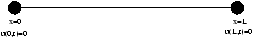
Figure 3.18 - For a Stretched String
now we try the type one solution
u(x,t)=(Ax+B)(Ct+D)
where (Ax+B)=X(x) so
X(0)=0=A0+B=B Þ B=0
X(L)=0=AL Þ A=0
this is the trivial solution u(x,t)=0 . This solution type is usually trivial however we will see in a later example that it is not always trivial.
now we try the type two solution
u(x,t)=(Acos(kx)+Bsin(kx))(Ccos(kct)+Dsin(kct))
where (Acos(kx)+Bsin(kx))=X(x) so
X(0)=0=A+B0=A Þ A=0
X(L)=Bsin(kL)=0
from the X(L) answer we have two choices
-
we could set B=0 and so we are back to the trivial solution from the type one solution
- make sin(kL)=0 which provides several repeating solutions
kL=np (n=integer)
this provides us with a discrete set of values for k , these are called eigenvalues.
Thus
the sin component is called an eigenfunction which is associated with the eigenvalue's k=np/L .
| u(x,t)=Bnsin |
|
æ
ç
ç
è |
Cncos |
|
+Dnsin |
|
|
ö
÷
÷
ø |
now we try the type three solution
X(x)=u(x,t)=Acosh(kx)+Bsinh(kx)
we get
X(0)=0=1A+B0=A Þ A=0
X(L)=0=Bsinh(kL)
B=0 Þ trivial solution
If we quickly summarise what we have done, for the solutions of
which satisies the homogenous boundary conditions (which are fixed ends of a string)
u(0,t)=0, u(L,t)=0
all these combine to produce
| u(x,t)=Bnsin |
|
æ
ç
ç
è |
Cncos |
|
+Dnsin |
|
|
ö
÷
÷
ø |
we now apply the inital conditions to obtain values for Bn , Cn and Dn .
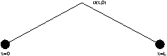
Figure 3.19 - The Initial Conditions of Our Fixed Ended String
also another initial condition that tells use the string starts off stationary
therefore
| |
|
=Bnsin |
|
é
ê
ê
ë |
Cn |
æ
ç
ç
è |
|
ö
÷
÷
ø |
æ
ç
ç
è |
-sin |
|
ö
÷
÷
ø |
+Dn |
æ
ç
ç
è |
|
ö
÷
÷
ø |
æ
ç
ç
è |
cos |
|
ö
÷
÷
ø |
ù
ú
ú
û |
=0 (at t=0) |
| 0=Bnsin |
|
é
ê
ê
ë |
Dn |
æ
ç
ç
è |
|
ö
÷
÷
ø |
ù
ú
ú
û |
Dn=0 |
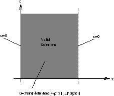
Figure 3.20 - Plots of Solutions in Regional Space
However in practice we are more likely to
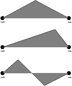
Figure 3.21 - Some Possible Practical Situations
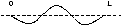
note the solution obtained (at t=0 ) is of the form Bnsin(np x/L)
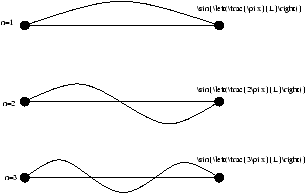
Figure 3-22 - Plausible Solutions
We note that we can can use any linear combination of the form
| B1sin |
|
cos |
|
+B2sin |
|
cos |
|
+B3sin |
|
cos |
|
+... |
| u(x,0)=B1sin |
|
+B2sin |
|
+B3sin |
|
+... |
3.4 Reminder about Fourier Series
For a periodic function f(x)=f(x+nx0) where the period is x0 . Any periodic function can be represented by an infinte series of the form
| f(x)= |
|
+ |
|
é
ê
ê
ë |
ancos |
|
+bnsin |
|
ù
ú
ú
û |
-
an :
- multiply by cos(2p px/x0) and integrate in the range -x0/2 to x0/2
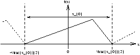
Figure 3.23 - Calculating the Fourier Constants
Noting these results
also that
so by doing all the integrations
so by changing p to n we can say
- a0 :
- from our work calculating an we obtain
- bn :
- multiply by sin(2p px/x0) and integrate in the range -x0/2 to x0/2
also that
and we obtain
The validities of this technique are
-
periodic function f(x) is
-
is continuous
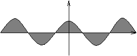
Figure 3.24 - Continuous Function
- or has a finite number (per period) of finite discontinuties
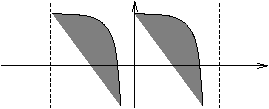
Figure 3.25 - Finite Number of Discontinuties
- can have discontinuties in the gradient
Figure 3.26 - Discontinuties in the Gradiant
At a discontinuity the fourier series tends to
Figure 3.27 - Discontinuity in Function
At a discontinuity in the gradient
Figure 3.28 - Discontinuity in Gradient
At a finite number of discontinuities
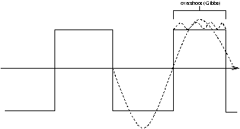
Figure 3.29 - Finite Number of Discontinies
If f(x) is not period but we choose a range (say) -x0/2<x<x0/2 we can construct a Fourier Series the standard way which is valid only for this range.
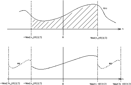
Figure 3.30 - Part of the Function
f(
x) as a Fourier Series
The Fourier Series over the complete range of x -¥<x<¥ , represents the functions f(x) in the range -x0/2<x<x0/2 periodically extended.
Special Results are obtained if f(x) is
-
even:
- f(-x)=f(x)
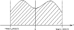
Figure 3.31 - An Even Function
consider
this is because the function is even so there are no contributing parts of sin
- odd:
- f(-x)=-f(x)
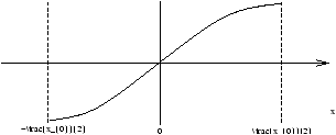
Figure 3.32 - An Odd Function
consider
also note that a0=0 too.
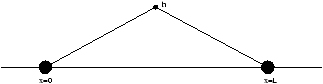
Figure 3.33 - Back to Our String Problem
this is inhomogeneous
We are now going to use
so the Fourier Series must only conatin sin terms
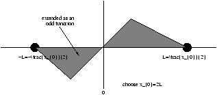
Figure 3.34 - The String as a Fourier Series
| f(x)= |
|
+ |
|
é
ê
ê
ë |
ancos |
|
+bnsin |
|
ù
ú
ú
û |
| bn= |
|
ó
õ |
|
fodd(x)sin |
|
dx=2 |
é
ê
ê
ê
ê
ê
ê
ê
ë |
|
ó
õ |
|
fodd(x)sin |
|
dx |
ù
ú
ú
ú
ú
ú
ú
ú
û |
For this case
| bn= |
|
ó
õ |
|
f(x)sin |
|
dx= |
|
ó
õ |
|
foddf(x)sin |
|
dx |
| bn=2 |
é
ê
ê
ê
ê
ê
ê
ê
ë |
|
ó
õ |
|
æ
ç
ç
è |
|
ö
÷
÷
ø |
sin |
|
dx+ |
|
ó
õ |
|
æ
ç
ç
è |
|
(L-x) |
ö
÷
÷
ø |
sin |
|
dx |
ù
ú
ú
ú
ú
ú
ú
ú
û |
| bn= |
é
ê
ê
ê
ê
ê
ê
ê
ê
ê
ê
ê
ë |
é
ê
ê
ê
ê
ê
ë |
|
|
ù
ú
ú
ú
ú
ú
û |
|
- |
ó
õ |
|
|
|
dx- |
ó
õ |
|
|
|
dx |
ù
ú
ú
ú
ú
ú
ú
ú
ú
ú
ú
ú
û |
| bn= |
|
é
ê
ê
ê
ê
ê
ê
ê
ê
ê
ê
ê
ê
ê
ê
ë |
|
|
|
-0+ |
é
ê
ê
ê
ê
ê
ê
ê
ê
ë |
|
|
ù
ú
ú
ú
ú
ú
ú
ú
ú
û |
|
+0-- |
|
|
|
- |
é
ê
ê
ê
ê
ê
ê
ê
ê
ë |
|
|
ù
ú
ú
ú
ú
ú
ú
ú
ú
û |
|
ù
ú
ú
ú
ú
ú
ú
ú
ú
ú
ú
ú
ú
ú
ú
û |
| n |
sin(np/2) |
| 1 |
1 |
| 2 |
0 |
| 3 |
-1 |
| 4 |
0 |
| |
| bn=2 |
é
ê
ê
ê
ê
ê
ê
ê
ë |
|
ó
õ |
|
æ
ç
ç
è |
|
ö
÷
÷
ø |
|
sin |
|
dx+ |
|
ó
õ |
|
æ
ç
ç
è |
|
(L-x) |
ö
÷
÷
ø |
sin |
|
dx |
ù
ú
ú
ú
ú
ú
ú
ú
û |
Bn=bn
this is only valid for 0<x<L and for t³ 0
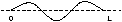
3.5 Wave on a String With Fixed Ends
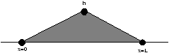
Figure 3.35 - Wave on a String
| Þ u(x,t)= |
|
é
ê
ê
ë |
|
× 1×sin |
|
cos |
|
+0- |
|
sin |
|
cos |
|
+0+ |
|
sin |
|
cos |
|
... |
ù
ú
ú
û |
| ct=L/4 |
ct=3L/4 |
 |
 |
| |
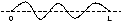
We note that in practice the loses are higher for higher order modes (frequencies) therefore this leaves only the fundemental or n=1 mode.
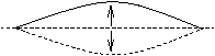
Figure 3.36 - The Fundemental Mode Remains
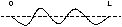
so why do we get
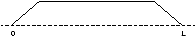
Figure 3.37 - The Strings Center is Flattened
we recall that
Þ sinA+sinB=2sinCcosD
where C+D=A and C-D=B
| sinCcosD= |
|
[ |
sin(C+D)+sin(C-D) |
] |
| Þ sin |
|
cos |
|
= |
|
é
ê
ê
ë |
sin |
|
+sin |
|
ù
ú
ú
û |
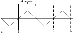
Figure 3.38 - Conversion to a Fourier Series
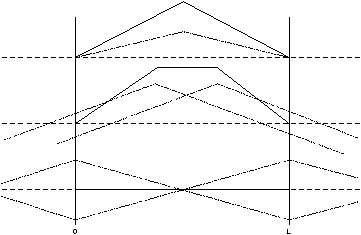
Figure 3.39 - Summation of Waves
3.6 d'Alemerts Solution to the Wave Equation
D. Alemberts (1717-1783) solution to the wave equation was (which we will be solving)
this is subject to u(x,0)=f(x) which describes the shape and the following equation is the transverse velocity
so the general solution we obtain is
u(x,t)=F(x+ct)+G(x-ct)
where F and G are arbitrary functions
u(x,0)=F(x)+G(x)=f(x)
we now put in that t=0
and now integrate with respect to x (the contents of the bracket)
| |
ó
õ |
|
F'(s)ds- |
ó
õ |
|
G'(s)ds= |
|
ó
õ |
|
g(s)ds |
| F(x)-F(a)-[G(x)-G(a)]= |
|
ó
õ |
|
g(s)ds |
F(x)+F(x)=f(x)
| F(x)-G(x)= |
|
ó
õ |
|
g(s)ds+[F(a)-G(a)] |
| F(x)= |
|
f(x)+ |
|
ó
õ |
|
g(s)ds+ |
|
[F(a)-G(a)] |
| G(x)= |
|
f(x)- |
|
ó
õ |
|
g(s)ds+ |
|
[F(a)-G(a)] |
u(x,t)=F(x+ct)+G(x-ct)
and the general solution is
| u(x,t)= |
|
[f(x+ct)+G(x-ct)]+ |
|
ó
õ |
|
g(s)ds |
we found that to satisfy the follow we require that f(x) is odd with a period of 2L
u(0,t)=0, u(L,t)=0
so the general solution gives the vibration of afixed string we took g(s)=0
3.7 Vibration of a Rectangular Drum
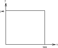
Figure 3.40 - A Rectangular Drum
u(x,y,t)=V(x,y)T(t)
likewise
and
we now substitute
we divide by u=VT
| |
|
æ
ç
ç
è |
|
+ |
|
ö
÷
÷
ø |
= |
|
× |
|
=seperation constant |
T''+k2c2T=0
T(t)=Ecos(kct)+Fsin(kct)
and for the left hand side
this is known as the Helmholtz Equation.
We now assume that V(x,y)=X(x)Y(y) so
X''Y+XY''+k2XY=0
divide by V=XY
the variables are seperable so
| |
|
æ
ç
ç
è |
|
ö
÷
÷
ø |
+ |
|
æ
ç
ç
è |
|
ö
÷
÷
ø |
+ |
|
(k2)=0 |
-kx2-ky2+k2=0
Þ k2=kx2+ky2
X(x)=Acos(kxx)+Bsin(kxx)
Y(y)=Ccos(kyy)+Dsin(kyy)
T(t)=Ecos(kct)+Fsin(kct)
now we apply our homogenous boundary conditions
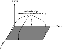
Figure 3.41 - The Boundary Condition of the Rectangular Drum
U=X(x)Y(y)T(t)
for when
x=0Þ u=0 so X(0)=0
x=aÞ u=0 so X(a)=0
therefore
X(0)=A+0Þ A=0
X(a)=0+Bsin(kxa)Þ A=0
so B=0 which is the trivial solution or the more interesting solution which is
likewise for the boundary condition Y(0)=0 and Y(b)=0 so
| U(x,y,t)=Bmsin |
|
Dnsin |
|
× |
é
ê
ê
ë |
Ecos |
|
+Fsin |
|
ù
ú
ú
û |
| u(x,y,t)=Bm,nsin |
|
sin |
|
×cos |
|
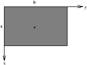
Figure 3.42 - The
m=1 and
n=1 Solution
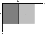
Figure 3.43 - The
m=1 and
n=2 Solution
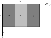
Figure 3.44 - The
m=1 and
n=3 Solution
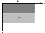
Figure 3.45 - The
m=2 and
n=1 Solution
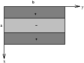
Figure 3.46 - The
m=3 and
n=1 Solution
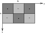
Figure 3.47 - The
m=2 and
n=3 Solution
These are normal modes of oscillation. The eigenfunctions from which we can construct a solution to satisfy the inhomogenous boundary conditions at t=0 . This involves
-
the shape of displacement
- u(x,y,0)=f(x,y)
so
To obtain the Fourier Series conatining only sin terms we need to extend f(x,y) as an odd function into the ranges -a<x<0 and -b<y<0 . So we put
thus we obtain
| Þ Cm(y)=2 |
é
ê
ê
ê
ê
ë |
|
ó
õ |
|
f(x,y)sin |
|
dx |
ù
ú
ú
ú
ú
û |
| Bm,n=2 |
é
ê
ê
ê
ê
ë |
|
ó
õ |
|
Cm(y)sin |
|
dy |
ù
ú
ú
ú
ú
û |
| Bm,n= |
|
ó
õ |
|
ó
õ |
|
f(x,y)sin |
|
sin |
|
dxdy |
3.8 The Heat Equation With Inhomogenous Boundary Conditions
Figure 3.48 - A Rod With a Temperature Distribution Across It
if u(0)=0 and u(L)=0 then the seperable solutions are
we now construct our solution
where
| Bn=2 |
é
ê
ê
ê
ê
ë |
|
ó
õ |
|
f(x)sin |
|
dx |
ù
ú
ú
ú
ú
û |
Figure 3.49 - A Different Set of Boundary Conditions
the inhomogenous boundary conditions are
u(0,t)=U0¹ 0
u(L,t)=UL¹ 0
u(x,t)=v(x)+w(x,t)
where v is the steady state function whilst w is the time varying one.
ie.
v(x)=Gx+H
the steady state part of the solution is
v(0)=U0=G.0+H (H=U0)
v(L)=UL=G.L+U0
Figure 3.50 - Plot Of The Steady State
we have
w(x,t)=u(x,t)-v(x)
we know that
u(0,t)=U0
u(L,t)=UL
w(0,t)=U0-U0=0
w(L,t)=UL-UL=0
w(x,t) satisifies the differential equation with the homogeneous boundary conditions
w(0,t)=0
w(L,t)=0
but u(x,0)=f(x) so
w(x,0)=u(x,0)-v(x)
| Þ w(x,0)=f(x)- |
æ
ç
ç
è |
|
ö
÷
÷
ø |
x-U0 |
| Bn=2 |
é
ê
ê
ê
ê
ë |
|
ó
õ |
|
æ
ç
ç
è |
f(x)- |
æ
ç
ç
è |
|
ö
÷
÷
ø |
x-U0 |
ö
÷
÷
ø |
sin |
|
dx |
ù
ú
ú
ú
ú
û |
3.9 Summary of Seperation of Variables
solving for example
-
u(x,t)=X(x)T(t)
- divide by U=XT (seperates the variables)
- choose the seperation constant ( 0 , ± k2 )
- look at the physics to help choose your seperation constant (we choose 0 and -k2 )
Þ X=Ax+B
Þ X=Acos(kx)+Bsin(kx)
- apply the homogenous boundary conditions. eg.
X(0)=0
X(L)=0
where n is an integer and k is a discrete set of eigenvalues with spacing p/L
therefore out solution is (the bit after Bn is the eigenfunction)
- we construct a linear combination of these eigenfunctions to satisify the inhomogenous boundary conditions. eg. u(x,0)=f(x)
- use a half range Fourier Series with f(x) extended as an odd function in the range -L<x<0
Figure 3.51 - Half Range Fourier Series
the period of the Fourier Series is 2L and the series represents f(x) extended as an odd function periodically extended for all x
The proceedure works because the function
are orthogonal over the range -L<x<L
3.10 Orthogonal Functions
A set of functions Un(x) are said to be orthogonal over a range a<x<b if
| |
ó
õ |
|
Um(x)Un(x)r(x)dx=0 m¹ n (or m=n¹ 0) |
Note that for sin(2p nx/x0) , etc we have r(x)=2 .
We can now represent f(x) in the range a£ x£ b as a sum of the orhogonal function Un
for example the Fourier Series
This is an example, there are many others such as
-
Legendre Polynomials
- Bessel Functions
3.11 Partial Differential Equations (Other Than The Cartesian Coordinate System)
the above is of the cartesian coordinate system, instead of this we will be looking at
-
plane polar coordinates
- cyclinderical polar coordinates
- spherical polar coordinates
3.11.1 Plane Polar Coordinates
(x,y)® (r,q )
0£ r<¥
-p£q£p
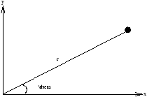
Figure 3.52 - Plane Polar Coordinates
Þ x=rcosq, y=rsinq
so we can obtain
so from r2=x2+y2
and also for
and from tanq=y/x
and the same is true for
now substituting into the original equation
we make this an operator
and its a similar process for y
we now need
| |
|
= |
æ
ç
ç
è |
cosq |
|
- |
|
|
ö
÷
÷
ø |
æ
ç
ç
è |
cosq |
|
- |
|
|
ö
÷
÷
ø |
| |
|
=cosq |
é
ê
ê
ë |
cosq |
|
- |
|
|
- |
|
|
- |
|
|
ù
ú
ú
û |
| |
|
= |
æ
ç
ç
è |
sinq |
|
+ |
|
|
ö
÷
÷
ø |
æ
ç
ç
è |
sinq |
|
+ |
|
|
ö
÷
÷
ø |
3.11.2 Cylindrical Polar Coordinates
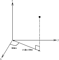
Figure 3.53 - Cylindrical Polar Coordinates
3.11.3 Spherical Polar Coordinates
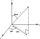
Figure 3.54 - Spherical Polar Coordinates
x,y,z® r,q ,f
z=rcosq
r =rsinq
x=rcosq
y=rsinq
from these results we can obtain
and by replacing x with z and y with r we obtain ¶2u/¶ z2+¶2u/¶r2 . Now by using our result from plane polar coordinates
and through similar means like before we obtain
we also have
x=rcosf, y=rsinf
and by using ¶2u/¶ x2+¶2u/¶ y2 we get
if we substitute for ¶ u/¶r
now if we add this to ¶2u/¶ z2+¶2u/¶f2
also we can get as an alternative version of Ñ2u
| Ñ2u= |
|
|
æ
ç
ç
è |
r2 |
|
ö
÷
÷
ø |
+ |
|
|
æ
ç
ç
è |
sinq |
|
ö
÷
÷
ø |
+ |
|
|
3.12 Laplace's Equation in Cyclindrical Polar Coordinates
Ñ2u=0
where u=u(r,f ,z)
We now assume that we can find a solution of the form
u(r,f ,z)=R(r)F (f )Z(z)
| R''F Z+ |
|
F Z+ |
|
F ''Z+RF Z''=0 |
F =Acos(kf )+Bsin(kf )
from symmetry
u(r,f ,z)=u(r,f +2p ,z)
so we obtain
F (f )=F (f +2p )
it is because of this cyclic symmetry we choose the seperation constant to be -k2
F =Acos[k(f +2p )]+Bsin[k(f +2p )]=Acos(kf )+Bsin(kf )
Þ k=n (integer)
now for the r terms
Þ r2R''+rR'-n2R=0
by substituting R=rm
Þ r2m(m-1)rm-2+rmrm-1-n2rm=0
Þ m(m-1)rm+mrm-n2rm=0
Þ (m(m-1)+m-n2)rm=0
(m2-n2)rm=0
m=± n
we discard 1/rn as it tends to infinity as r® 0
u(r,f )=rn(Acos(nf )+Bsin(nf ))
| u(r,f )=rn |
( |
Ancos(nf )+Bnsin(nf ) |
) |
F ''+kF =0®F ''=0
F '=Cf +D
but we require that the solution is symmetric
F (f)=F (f +2p )® C=0
| Þ u(r,f )=A+ |
|
rn |
( |
Ancos(nf )+Bnsin(nf ) |
) |
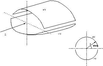
Figure 3.55 - A Split Conductor (aka capacitor)
Figure 3.56 -
u(
r,
f )
® u(
a,
f )=
f(
f )
As f(f ) is odd when we construct the Fourier Series we get A0=0 and An=0 so we obtain
| f(f )= |
|
bnsin(nf ) (standard fourier series) |
| bn=2 |
é
ê
ê
ê
ê
ë |
|
ó
õ |
|
Vsin(nf )df |
ù
ú
ú
ú
ú
û |
= |
|
é
ê
ê
ë |
|
ù
ú
ú
û |
|
= |
|
é
ê
ê
ë |
|
- |
|
ù
ú
ú
û |
Bnan=bn
| Þ u(r,f )= |
|
|
|
æ
ç
ç
è |
|
ö
÷
÷
ø |
|
sin(nf ) |
3.12.1 Vibration of a Circular Drum
we choose our function of u to be u=u(r,f ,t) (in plane polar coordinates)
u(r,f ,t)=R(r)F (f)T(t)
now by dividing by U=RF T
We know we are looking for a oscilating solution and so we use the seperation constant -k2=1/c2T''/T
T''+k2c2T=0
T(t)=Ecos(kct)+Fsin(kct)
we now notice that w =kc if we are looking of a oscilating solution (of which we are). This leaves
now by multiplying r2
we can now easily seperate the variables, so we put
As we require that there is symmetry (ie. F (f )=F (f +2p) )
So far our solution is
| u(r,f ,t)=R(r) |
( |
Ccos(nf )+Dsin(nf ) |
) |
× |
( |
Ecos(kct)+Fsin(kct) |
) |
--------
Note that if we differentiated, so
--------
where k2 is associated with the variation of time and n2 is the ??germination?? This is Bessel's Equation, however we are used to seeing it in terms of x and y . So if we put R=y and rk=x
Þ x2y''+xy'+(x2-n2)y=0
n is the general Bessel Equation and doesn't have to be an integer, however in our case n =n=integer .
This has solutions (we expect two solutions due to the differential equation being second order)
so when n is equal to an integer (ie. n ) then
J-n(x)=(-1)nJn(x)
so our solutions are linearly dependent and so we only can directly obtain one solution. So to get our second solution we use altering equation
y(x)=AJn(x)+BYn(x)
where AJn(x) is the first kind solution whilst BYn(x) is the second kind solution.
Figure 3.57 - Plots of Our Solutions
For a circular drum of radius a
includegraphics[scale=0.5]figures/eps/3-58.eps
Figure 3.58 - A Circular Drum ( R(a)=0 )
we know that R(r)=Jn(kr)
u=Jn(kr)(Ccos(nf )+Dsin(nf ))(Ecos(kct)+Fsin(kct))
we remember also that kc=w .
At r=a
Jn(ka)=0
For example
| |
m=1 |
m=2 |
m=3 |
m=4 |
| J0=0 (n=0) |
2.404 |
5.520 |
8.654 |
11.792 |
| J1=0 (n=1) |
3.832 |
7.016 |
10.173 |
13.323 |
| |
Let the zeros of Jn(x) be an,m (eg. a0,1=2.404 , etc) where n is the order of the Bessel Function and m is the number to identify which zero is being referenced to.
We require that
ka=an,m
this is because w=kc .
We now consider that n=0 which implies that there is no angular variation. We recall that our Bessel function is doing and and we note that J0(a0,m) are orthogonal.
Figure 3.59 - Recalling Our Bessel Function
so when m=1
Figure 3.60 - The Drum Solution For When
n=0 and
m=1
when m=2
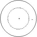
Figure 3.61 - The Drum Solution For When
n=0 and
m=2
when m=3
Figure 3.62 - The Drum Solution For When
n=0 and
m=3
now we look at n=1 so when m=1
Figure 3.63 - The Drum Solution For When
n=1 and
m=1
and when m=2
Figure 3.64 - The Drum Solution For When
n=1 and
m=2
In general we need a mixture of these modes to satisify the initial conditions, we use a double series (using k=an,m/a )
| u(r,f ,t)= |
|
|
Jn |
æ
ç
ç
è |
an,m |
|
ö
÷
÷
ø |
(Cn,mcos(nf )+Dn,msin(nf ))(En,mcos(kct)+Fn,msin(kct)) |
| |
ó
õ |
|
rJn |
æ
ç
ç
è |
an,m' |
|
ö
÷
÷
ø |
Jn |
æ
ç
ç
è |
an,m |
|
ö
÷
÷
ø |
dr=0 (m¹ m') |
| |
ó
õ |
|
rJn |
æ
ç
ç
è |
an,m' |
|
ö
÷
÷
ø |
Jn |
æ
ç
ç
è |
an,m |
|
ö
÷
÷
ø |
dr= |
|
[ |
Jn+1(an,m) |
] |
(m=m') |
3.13 Spherical Polor Coordinates
Lapaces Equation Ñ2u=0 and u=u(r,q ,f )
| |
|
|
æ
ç
ç
è |
r |
|
ö
÷
÷
ø |
+ |
|
|
æ
ç
ç
è |
sinq |
|
ö
÷
÷
ø |
+ |
|
|
=0 |
In the general case
u(r,q ,f )=R(r)Y(q ,f )
| |
|
|
æ
ç
ç
è |
r2 |
|
ö
÷
÷
ø |
Y+ |
|
|
æ
ç
ç
è |
sinq |
|
ö
÷
÷
ø |
+ |
|
|
=0 |
| |
|
|
æ
ç
ç
è |
sinq |
|
ö
÷
÷
ø |
+ |
|
|
=- |
|
|
æ
ç
ç
è |
r2 |
|
ö
÷
÷
ø |
The angular part becomes
| |
|
|
æ
ç
ç
è |
sinq |
|
ö
÷
÷
ø |
+ |
|
|
+l(l+1)Y=0 |
| |
|
|
|
æ
ç
ç
è |
sinq |
|
ö
÷
÷
ø |
+ |
|
|
+l(l+1)=0 |
| |
|
|
æ
ç
ç
è |
sinq |
|
ö
÷
÷
ø |
+l(l+1)sin2q=- |
|
Þ F ''+m2F=0
we note that if m=0 then we get an unsuitable solution ( F =CF +D ) so we ignore it. However when m 0 then we obtain
as we require symmetry ( F (f )=F (f +2p ) ) we discover that m must be an integer.
we now substiture -m2 into out q equation and divide by sin2q
| |
|
|
æ
ç
ç
è |
sinq |
|
ö
÷
÷
ø |
+ |
é
ê
ê
ë |
l(l+1)- |
|
ù
ú
ú
û |
Q =0 |
| |
|
é
ê
ê
ë |
(1-x2) |
|
ù
ú
ú
û |
+ |
é
ê
ê
ë |
l(l+1)- |
|
ù
ú
ú
û |
Q =0 |
If m=0 then we obtain the Legendre Equation
and when m 0 then we obtain the Associate Legendre Equation
| (1-x2) |
|
-2x |
|
+ |
é
ê
ê
ë |
l(l+1)- |
|
ù
ú
ú
û |
Q =0 |
3.13.1 Legendre Equation
The solution for an integer l exists in the range -1£ x£ 1 . The solutions are then polynominals ( Pl(x) ), for example
-
P0(x)=1
- P1(x)=x
- P2(x)=1/2(3x2-1)
with the Associate Legendre Equation
we therefore have for the spherical problem
| Yl,-m(q ,f )=Pl-m(cosq |
)e |
|
So our total solution is
| u(r,q ,f )= |
æ
ç
ç
è |
Arl+ |
|
ö
÷
÷
ø |
( |
CYl,m(q ,f )+DYl,-m(q ,f ) |
) |
We now integrate this from x=a to x=b
| |
ó
õ |
|
|
[p(unum'-umun')]dx+(lm-ln) |
ó
õ |
|
r(x)um(x)un(x)dx |
p[unum'-umun']ab
This relates to the value of this expression at the ends of the range ( x=a and x=b ). We can choose this part of the integral to equal zero.
p(b)[un(b)um'(b)-um(b)un'(b))]-p(a)[un(a)um'(a)-um(a)un'(a))]=0
If this is satisified then
| (lm-ln) |
ó
õ |
|
r(x)um(x)un(x)dx=0 |
p(b)[un(b)um'(b)-um(b)un'(b))]-p(a)[un(a)um'(a)-um(a)un'(a))]=0
There are several ways of ensuring this condition
-
make um(a)=um(b)=0 for all values of m (and also n ), this is known as a periodic boundary condition
- make um'(a)=um'(b)=0 again for all values of m (and n )
- make um'(a)+a u(a)=0 and um'(b)+b u(b)=0 for all values of m (and n )
Þ un(a)um'(b)-um(a)un'(a)=un(a)(-a un(a))-um(a)(-a un(a)=0
and this process can be repeated for the b extreme.
Subject to these conditions of the value of u and u' at the end of the range a to b , we can represent any function.
The values of an are derived using the orthogonality relationship. To do this we multiply this equation by um(x)r(x) (must include the weight function) and then we integrate across the range a to b .
| |
ó
õ |
|
f(x)r(x)um(x)dx= |
|
an |
ó
õ |
|
um(x)un(x)r(x)dx |
| |
ó
õ |
|
f(x)r(x)um(x)dx=an |
ó
õ |
|
um(x)un(x)r(x)dx |
| |
ó
õ |
|
um(x)un(x)r(x)dx=0,1 (m n;m=n) |
3.14 Series Solution of Differential Equations
Note that we already have done this for y''+y=0 .
3.14.1 Legendre's Equation
(1-x2)y''-2xy'+l(l+1)y=0
we expect that something special will occur at x=± 1 as the first term will disappear. We firstly assume that
| y=a0+a1x+a2x2+a3x3+... = |
|
anxn |
| Þ y'=0+a1+2a2x+3a3x2+... = |
|
nanxn-1 |
| Þ y''=0+0+2a2+3.2a3x+... = |
|
n(n-1)anxn-2 |
(1-x2)y''-2xy'+l(l+1)y=0
| |
|
n(n+1)anxn-2- |
|
n(n-1)anxn-2 |
|
nanxn+l(l+1) |
|
anxn=0 |
Þ 2(2-1)a2+0-0+l(l+1)a0=0
and at p=1 where we obtain the x1
Þ 3(3-1)a3+0-2.1a1+l(l+1)a1=0
and when p³ 2
Þ (p+2)(p+1)ap+2-p(p-1)ap-2pap+l(l+1)ap=0
(p+2)(p+1)ap+2=[p(p-1)+2p-l(l+1)]ap
(p+2)(p+1)ap+2=[p2-l2+p-l]ap
(p+2)(p+1)ap+2=-(l-p)(l+p+1)ap
we now have
also
and similarly
we now substitute for a2
| a4= |
| (l-2)(l)(l+1)(l+3) |
|
| 4.3.2.1 |
|
a0 |
| a5=- |
|
a3=- |
| (l-3)(l-1)(l+2)(l+4) |
|
| 5.4.3.2.1 |
|
a1 |
| y(x)=a0 |
é
ê
ê
ë |
1- |
|
x2+ |
|
x4+... |
ù
ú
ú
û |
+a1 |
é
ê
ê
ë |
x- |
|
x3+ |
|
x5+... |
ù
ú
ú
û |
y(x)=a0y1(x)+a1y2(x)
These are linearly independent solutions. We now need to investigate the range of values of x for which these two solutions y1(x) and y2(x) converge.
We use the Ratio Test for any series where for the series å up we look at
however we need to consider
so we look at
| |
|
½
½
½
½ |
|
½
½
½
½ |
= |
|
½
½
½
½ |
|
x2 |
½
½
½
½ |
<1 (to converge) |
We now set up the polynominal Pl(x) such that Pl(1)=1 so that when
l=0Þ y1=1, P0(x)=1
l=1Þ y2=x, P1(x)=x
| l=2Þ y1=1-3x, P2(x)= |
|
(3x2-1) |
| l=3Þ y2=x- |
|
, P3(x)= |
|
(5x3-3x) |
3.15 The Gamma (or Factorial) Function
we define the gamma function ( G ) as
so when x=x+1 we obtain
| G (x+1)= |
ó
õ |
|
e-ttxdt= |
[ |
-e-ttx |
] |
|
- |
ó
õ |
|
-e-txtx-1dt=0+xG (x) |
G (x+1)=xG (x)
also we notice that
| G (1)= |
ó
õ |
|
e-tdt= |
[ |
-e-t |
] |
|
=--1 |
Þ G (1)=1
and the same sort of thing applies for x=2,3,4,...
G (2)=G (1+1)=1G (1)=1
G (3)=G (2+1)=2G (2)=2.1
G (4)=G (3+1)=3G (3)=3.2.1
so the general patteren is
G (n+1)=n!
so it follows that
G (0+1)=0!=1
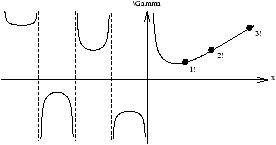
Figure missing.2 - Plot of the Gamma Function